Summarizing Numerical Associations

STAT 20: Introduction to Probability and Statistics

Adapted by Gaston Sanchez

Agenda

• Announcements
• Concept Questions
• Worksheet
• Break
• Lab 2.2 (extended): Computing on The Data

Announcements

• Reading Questions

• Lab 2.2

• Worksheet

Concept Questions

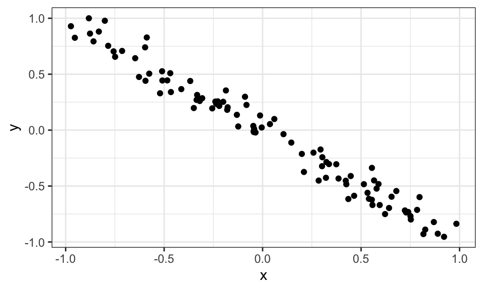
Estimate the correlation

countdown::countdown(1, top = 0)

01:00

What is the (Pearson) correlation coefficient between these two variables?

n_samples <- 100
set.seed(1)
x <- runif(n = n_samples, min = -1, max = 1) 
y <- -x + rnorm(n = n_samples, mean = 0, sd = .1)

data.frame(x = x, 
           y = y) |> 
  ggplot(aes(x = x, y = y)) +  
  geom_point() +
  theme_bw()

This plot has a strong negative linear association, so the correlation coefficient will be around -.8 or -.9.

The goal of this exercise is threefold: - Start calibrating the ability to associate the correlation with the structure in a scatter plot. - Make it clear that this is still just an informal eye-balling procedure (therefore multiple answers can be reasonable, but some are un-reasonable). - Set some of them up for a challenge on the next one; some will conflate correlation with association.

# simulate data -----------------------------------------------------
set.seed(9274)

x1 <- seq(0, 6, by = 0.05)

y_u <- (x1-3)^2 - 4 + rnorm(length(x1), mean = 0, sd = 1)
y_lin_pos_strong <- 3*x1 + 10 + rnorm(length(x1), mean = 0, sd = 2)
y_lin_pos_weak <- 3*x1 + 10 + rnorm(length(x1), mean = 0, sd = 20)

x2 <- seq(-8, -2, by = 0.05)

y_n <- -1 * (x2 + 5)^2 + 1 + rnorm(length(x2), mean = 0, sd = 2)
y_lin_neg_strong <- -5 * x2 + 3 + rnorm(length(x2), mean = 0, sd = 2)
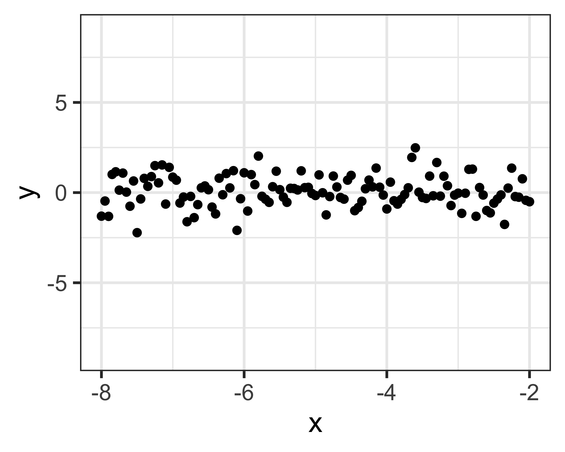
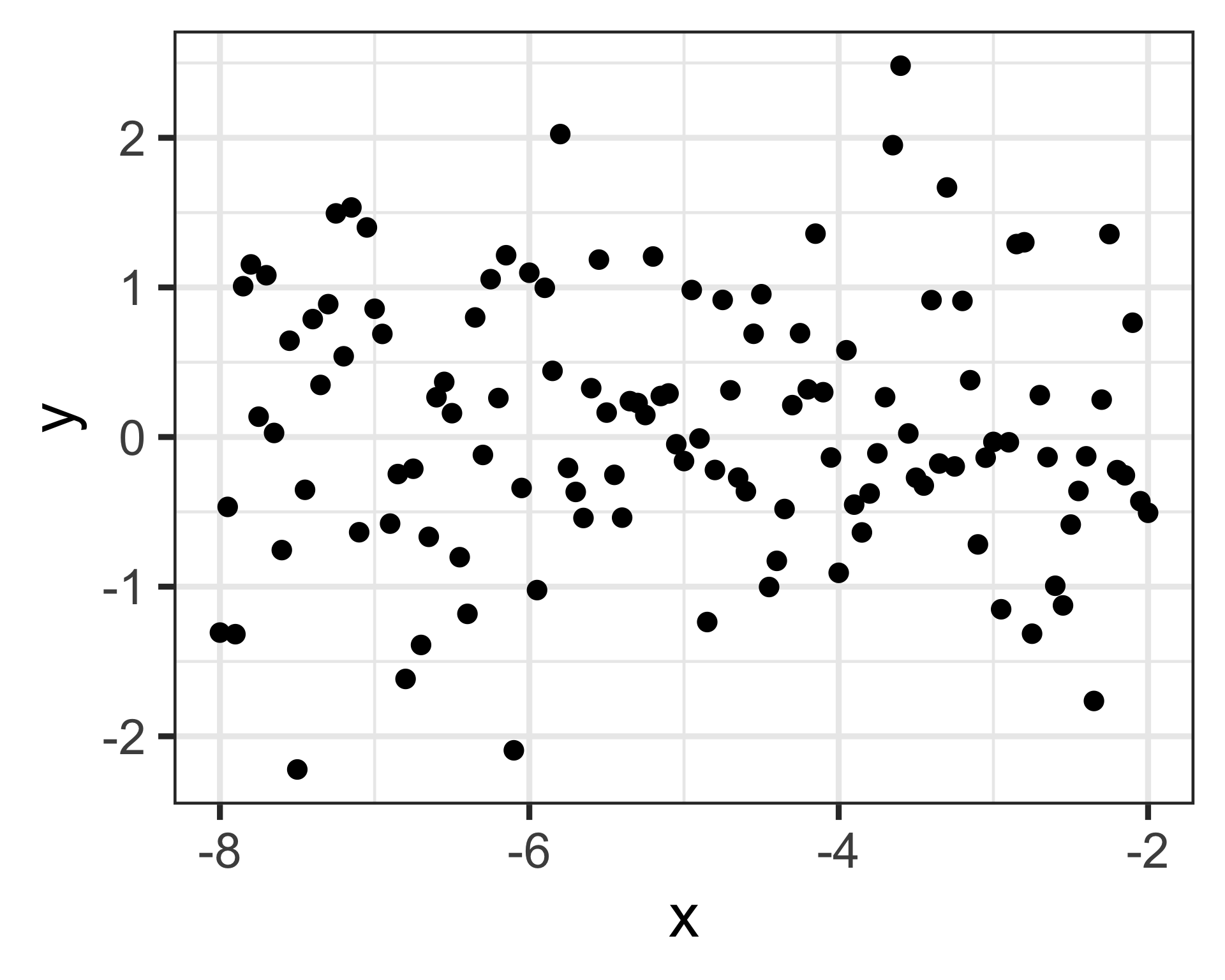
y_none <- rnorm(length(x2), mean = 0, sd = 1)

df <- data.frame(x = c(rep(x1, 3), rep(x2, 3)),
                 y = c(y_u, y_lin_pos_strong, y_lin_pos_weak,
                       y_n, y_lin_neg_strong, y_none),
                 plot_num = rep(LETTERS[1:6], each = length(x1)))

library(tidyverse)
pa <- df |>
    filter(plot_num == "A") |>
    ggplot(aes(x = x, 
               y = y)) +
    geom_point() +
    facet_wrap(vars(plot_num), scales = "free") +
    theme_bw(base_size = 14) +
    theme(axis.text.x=element_blank(),
          axis.ticks.x=element_blank(),
          axis.text.y=element_blank(),
          axis.ticks.y=element_blank()) +
    labs(x = "",
         y = "")

pb <- df |>
    filter(plot_num == "B") |>
    ggplot(aes(x = x, 
               y = y)) +
    geom_point() +
    facet_wrap(vars(plot_num), scales = "free") +
    theme_bw(base_size = 14) +
    theme(axis.text.x=element_blank(),
          axis.ticks.x=element_blank(),
          axis.text.y=element_blank(),
          axis.ticks.y=element_blank()) +
    labs(x = "",
         y = "")

pc <- df |>
    filter(plot_num == "C") |>
    ggplot(aes(x = x, 
               y = y)) +
    geom_point() +
    facet_wrap(vars(plot_num), scales = "free") +
    theme_bw(base_size = 14) +
    theme(axis.text.x=element_blank(),
          axis.ticks.x=element_blank(),
          axis.text.y=element_blank(),
          axis.ticks.y=element_blank()) +
    labs(x = "",
         y = "")

pd <- df |>
    filter(plot_num == "D") |>
    ggplot(aes(x = x, 
               y = y)) +
    geom_point() +
    facet_wrap(vars(plot_num), scales = "free") +
    theme_bw(base_size = 14) +
    theme(axis.text.x=element_blank(),
          axis.ticks.x=element_blank(),
          axis.text.y=element_blank(),
          axis.ticks.y=element_blank()) +
    labs(x = "",
         y = "")

pe <- df |>
    filter(plot_num == "E") |>
    ggplot(aes(x = x, 
               y = y)) +
    geom_point() +
    facet_wrap(vars(plot_num), scales = "free") +
    theme_bw(base_size = 14) +
    theme(axis.text.x=element_blank(),
          axis.ticks.x=element_blank(),
          axis.text.y=element_blank(),
          axis.ticks.y=element_blank()) +
    labs(x = "",
         y = "")

pf <- df |>
    filter(plot_num == "F") |>
    ggplot(aes(x = x, 
               y = y)) +
    geom_point() +
    facet_wrap(vars(plot_num), scales = "free") +
    theme_bw(base_size = 14) +
    ylim(-9, 9) +
    theme(axis.text.x=element_blank(),
          axis.ticks.x=element_blank(),
          axis.text.y=element_blank(),
          axis.ticks.y=element_blank()) +
    labs(x = "",
         y = "")

library(patchwork)
(pa + pb + pc) / (pd + pe + pf)

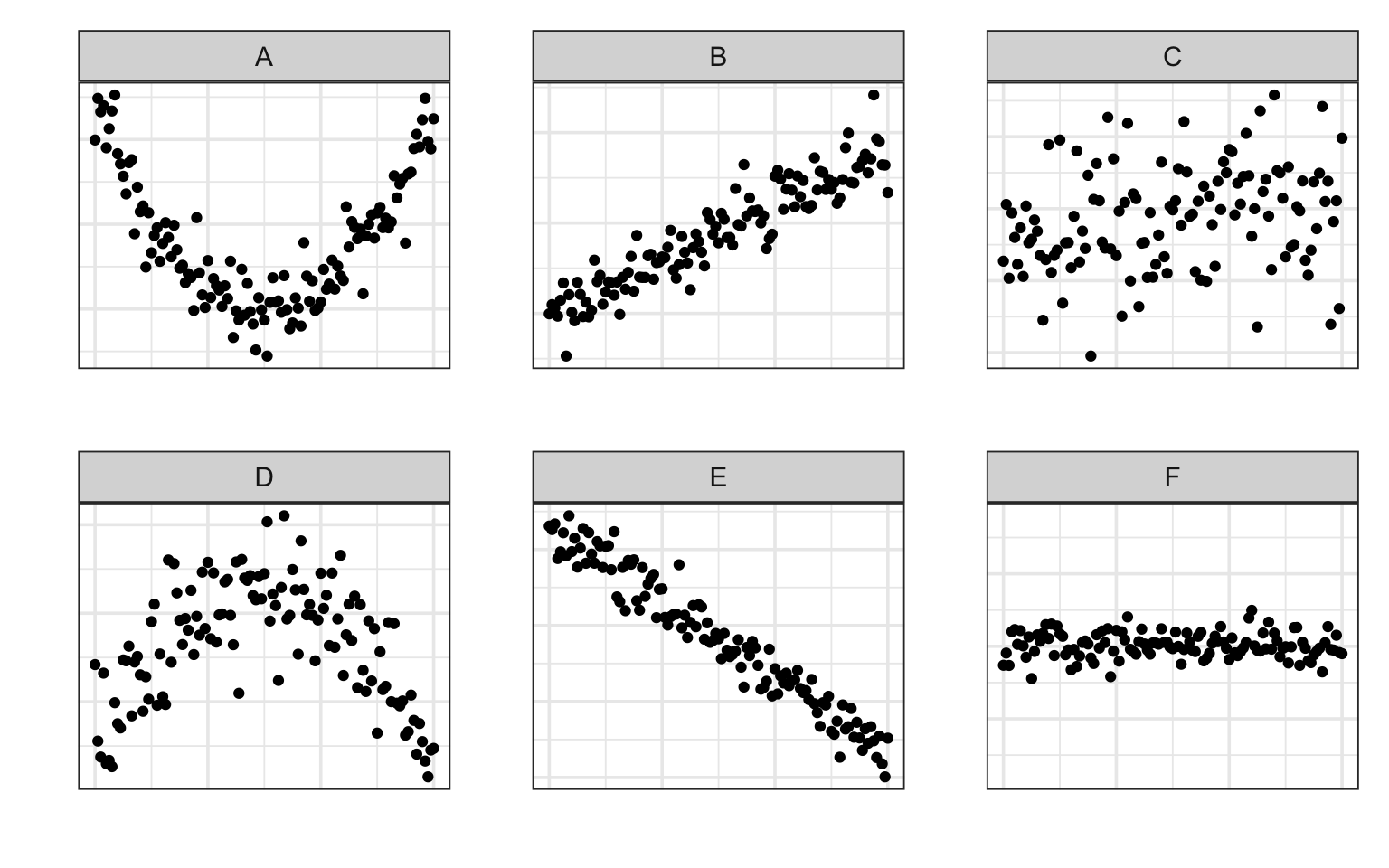
Which four plots exhibit the strongest association?

countdown::countdown(1, top = 0)

01:00

Student will likely identify A, B, E, and F. F only appears to be highly associated because of the scaling of the y-axis. This is a good opportunity to review definition of association. The following slides demonstrate the effects of that scaling.

Correlation and Scale

df_f

Pearson Correlation and Scale

df_f

        x            y
1   -8.00 -1.307007369
2   -7.95 -0.466886973
3   -7.90 -1.317638373
4   -7.85  1.008059015
5   -7.80  1.153714017
6   -7.75  0.136000314
7   -7.70  1.081268517
8   -7.65  0.027234440
9   -7.60 -0.755489564
10  -7.55  0.643581028
11  -7.50 -2.221816425
12  -7.45 -0.352711462
13  -7.40  0.788325702
14  -7.35  0.348209977
15  -7.30  0.888132692
16  -7.25  1.494640228
17  -7.20  0.539665177
18  -7.15  1.534245783
19  -7.10 -0.636288267
20  -7.05  1.400750746
21  -7.00  0.857266821
22  -6.95  0.689240640
23  -6.90 -0.578689332
24  -6.85 -0.247484190
25  -6.80 -1.616711187
26  -6.75 -0.211921880
27  -6.70 -1.389650022
28  -6.65 -0.667030427
29  -6.60  0.265923179
30  -6.55  0.368512913
31  -6.50  0.159370185
32  -6.45 -0.803029578
33  -6.40 -1.181853575
34  -6.35  0.799141786
35  -6.30 -0.119741600
36  -6.25  1.055099362
37  -6.20  0.260610303
38  -6.15  1.215058556
39  -6.10 -2.093776227
40  -6.05 -0.340475843
41  -6.00  1.098181964
42  -5.95 -1.022920292
43  -5.90  0.997308309
44  -5.85  0.442282185
45  -5.80  2.024841893
46  -5.75 -0.206236931
47  -5.70 -0.366921396
48  -5.65 -0.540982671
49  -5.60  0.326545855
50  -5.55  1.185875818
51  -5.50  0.163270582
52  -5.45 -0.252746010
53  -5.40 -0.538783647
54  -5.35  0.239830058
55  -5.30  0.227238979
56  -5.25  0.146973095
57  -5.20  1.206565164
58  -5.15  0.274237725
59  -5.10  0.291223416
60  -5.05 -0.048435420
61  -5.00 -0.160503335
62  -4.95  0.982662625
63  -4.90 -0.009812706
64  -4.85 -1.236449694
65  -4.80 -0.220086594
66  -4.75  0.916450245
67  -4.70  0.312158589
68  -4.65 -0.271222289
69  -4.60 -0.362834150
70  -4.55  0.690127669
71  -4.50  0.954579372
72  -4.45 -1.002334741
73  -4.40 -0.827510811
74  -4.35 -0.481050964
75  -4.30  0.213284850
76  -4.25  0.694018655
77  -4.20  0.318705891
78  -4.15  1.359291786
79  -4.10  0.299499214
80  -4.05 -0.136853535
81  -4.00 -0.907524278
82  -3.95  0.580039124
83  -3.90 -0.451761432
84  -3.85 -0.637651429
85  -3.80 -0.377287558
86  -3.75 -0.108975033
87  -3.70  0.266174878
88  -3.65  1.950537958
89  -3.60  2.481797153
90  -3.55  0.024020307
91  -3.50 -0.271974465
92  -3.45 -0.324420253
93  -3.40  0.914990966
94  -3.35 -0.177070403
95  -3.30  1.668125591
96  -3.25 -0.196626395
97  -3.20  0.909735944
98  -3.15  0.379802619
99  -3.10 -0.717674077
100 -3.05 -0.137978296
101 -3.00 -0.032596143
102 -2.95 -1.151078285
103 -2.90 -0.035147120
104 -2.85  1.289653594
105 -2.80  1.301664628
106 -2.75 -1.314453018
107 -2.70  0.279983464
108 -2.65 -0.134496134
109 -2.60 -0.993968666
110 -2.55 -1.125493956
111 -2.50 -0.585075814
112 -2.45 -0.360440229
113 -2.40 -0.128946258
114 -2.35 -1.763949074
115 -2.30  0.249921212
116 -2.25  1.356315758
117 -2.20 -0.221241869
118 -2.15 -0.255945298
119 -2.10  0.764032808
120 -2.05 -0.429023148
121 -2.00 -0.506416626

Pearson Correlation and Scale

df_f |>
    ggplot(aes(x = x,
               y = y)) +
    geom_point() +
    ylim(-9, 9) +
    theme_bw()

Pearson Correlation and Scale

df_f |>
    ggplot(aes(x = x,
               y = y)) +
    geom_point() +
    ylim(-9, 9) +
    theme_bw()

Pearson Correlation and Scale

df_f |>
    ggplot(aes(x = x,
               y = y)) +
    geom_point() +
    theme_bw()

Pearson Correlation and Scale

df_f |>
    ggplot(aes(x = x,
               y = y)) +
    geom_point() +
    theme_bw()

Pearson Correlation and Scale

df_f |>
    summarize(pearson = cor(x, y))

Pearson Correlation and Scale

df_f |>
    summarize(pearson = cor(x, y))

      pearson
1 -0.03106456

Describing Associations

When considering the structure in a scatter plot, pay attention to:

1. The strength of the association
   • How much does the conditional distribution of y change when you move along the x?

2. The shape of the association
   • Linear? Quadratic? Cubic or beyond?

3. The direction of the (linear) association
   • Positive or negative?

WS: Summarizing Numerical Associations

25:00

Break

05:00

Lab 2.2 (extended): Computing on The Data

35:00

End of Lecture