Multiple Linear Regression

STAT 20: Introduction to Probability and Statistics

Adapted by Gaston Sanchez

Agenda

• Announcements

• Linear Regression Refresher

  • Simple Linear Regression
  • Multiple Linear Regression

• Practice Problems on Regression

• Lab 3.2 Flights

Announcements: Quiz 2

Quiz-2 next Monday, Sep 29th in class.

• Section 1, 8am in Barker 101
• Section 8, 10am in SOCS 60

• Topics:
  • Summarizing Numerical Data
  • A Grammar of Graphics
  • Conditioning
  • Summarizing Associations
  • Multiple Linear Regression

Linear Regression Refresher

Simple Linear Regression Models in R

Function lm()

# simple linear regression
mod <- lm(formula = y ~ x, data = dataset)

• y: response variable
• x: predictor variable
• data: name of data frame

• coefficients(mod): regression coeffs
• fitted(mod): predicted values
• residuals(mod): residuals

Multiple Linear Regression Models in R

Function lm()

# multiple linear regression
mod <- lm(formula = y ~ x1 + x2 + ..., data = dataset)

• y: response variable
• x1, x2, ...: predictor variables
• data: name of data frame

• coefficients(mod): regression coeffs
• fitted(mod): predicted values
• residuals(mod): residuals

Examples

Penguins Data

penguins |> 
  select(c(1:4, 6:7)) |> 
  slice_sample(n = 5)

# A tibble: 5 × 6
  species island bill_length_mm bill_depth_mm body_mass_g sex   
  <fct>   <fct>           <dbl>         <dbl>       <int> <fct> 
1 Adelie  Dream            36.3          19.5        3800 male  
2 Adelie  Biscoe           41.4          18.6        3700 male  
3 Gentoo  Biscoe           43.6          13.9        4900 female
4 Gentoo  Biscoe           45.5          13.9        4200 female
5 Gentoo  Biscoe           46.5          14.8        5200 female

Simple Regression: 2 numerical

Simple Regression: 2 numerical

# model 1
m1 <- lm(formula = bill_depth_mm ~ bill_length_mm, data = penguins)
m1

Call:
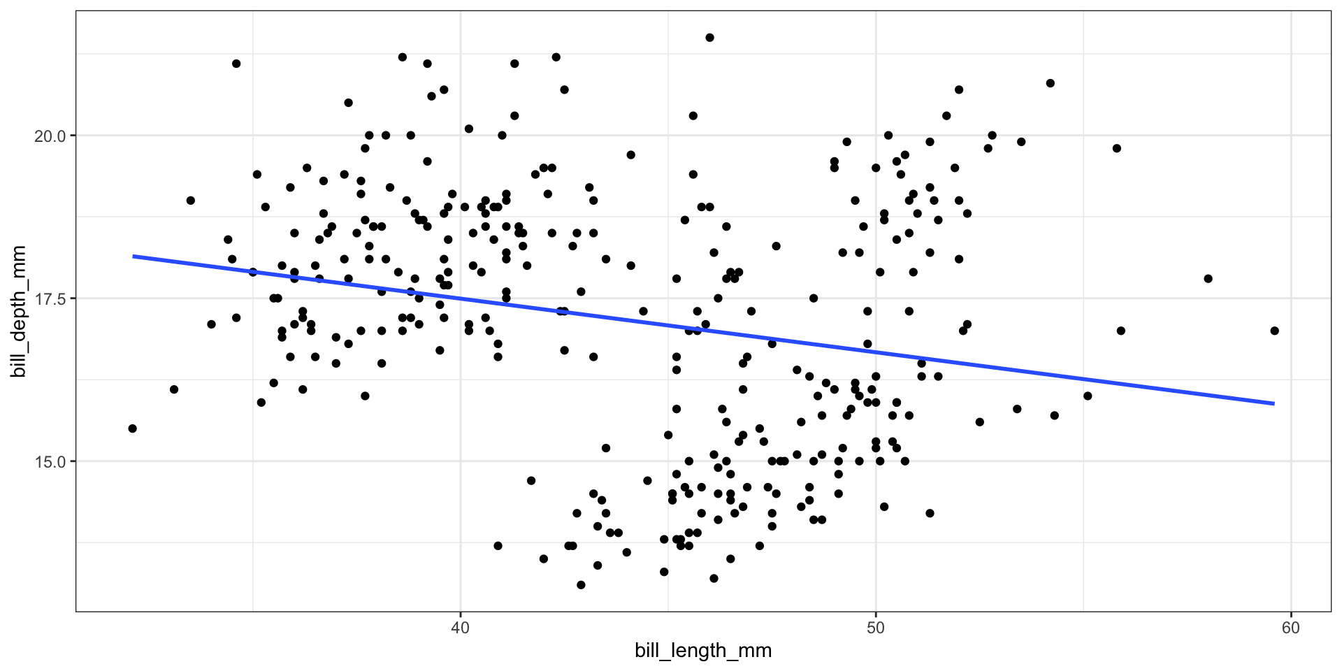
lm(formula = bill_depth_mm ~ bill_length_mm, data = penguins)

Coefficients:
   (Intercept)  bill_length_mm  
      20.78665        -0.08233  

\[ \widehat{\texttt{bill_depth_mm}} = 20.786 -0.0823 \ \texttt{bill_length_mm} \]

Simple Regression: 2 numerical

# model 1
m1 <- lm(formula = bill_depth_mm ~ bill_length_mm, data = penguins)
m1

Call:
lm(formula = bill_depth_mm ~ bill_length_mm, data = penguins)

Coefficients:
   (Intercept)  bill_length_mm  
      20.78665        -0.08233  

01:00

How can we interpret the coefficient associated to bill_length_mm?

Simple Regression: 2 numerical

# model 1
m1 <- lm(formula = bill_depth_mm ~ bill_length_mm, data = penguins)
m1

Call:
lm(formula = bill_depth_mm ~ bill_length_mm, data = penguins)

Coefficients:
   (Intercept)  bill_length_mm  
      20.78665        -0.08233  

For every additional millimeter in bill length, we expect bill depth to decrease by 0.08233 millimeters.

Multiple Regression: 3 numerical

Multiple Regression: 3 numerical

# model 2
m2 <- lm(formula = bill_depth_mm ~ bill_length_mm + body_mass_g, 
         data = penguins)
m2

Call:
lm(formula = bill_depth_mm ~ bill_length_mm + body_mass_g, data = penguins)

Coefficients:
   (Intercept)  bill_length_mm     body_mass_g  
     21.278127        0.027373       -0.001264  

\[ \widehat{\texttt{bill_depth_mm}} = 21.278 + 0.0273 \ \texttt{bill_length_mm} \\ - 0.0012 \ \texttt{body_mass_g} \]

Multiple Regression: 3 numerical

# model 2
m2 <- lm(formula = bill_depth_mm ~ bill_length_mm + body_mass_g, 
         data = penguins)
m2

Call:
lm(formula = bill_depth_mm ~ bill_length_mm + body_mass_g, data = penguins)

Coefficients:
   (Intercept)  bill_length_mm     body_mass_g  
     21.278127        0.027373       -0.001264  

01:00

How can we interpret the coefficient associated to bill_length_mm?

Multiple Regression: 3 numerical

# model 2
m2 <- lm(formula = bill_depth_mm ~ bill_length_mm + body_mass_g, 
         data = penguins)
m2

Call:
lm(formula = bill_depth_mm ~ bill_length_mm + body_mass_g, data = penguins)

Coefficients:
   (Intercept)  bill_length_mm     body_mass_g  
     21.278127        0.027373       -0.001264  

For penguins of the same body mass, an additional millimeter in bill length is associated with an increase of 0.0273 millimeters in bill depth.

Multiple Regression: 3 numerical

# model 2
m2 <- lm(formula = bill_depth_mm ~ bill_length_mm + body_mass_g, 
         data = penguins)
m2

Call:
lm(formula = bill_depth_mm ~ bill_length_mm + body_mass_g, data = penguins)

Coefficients:
   (Intercept)  bill_length_mm     body_mass_g  
     21.278127        0.027373       -0.001264  

01:00

How can we interpret the coefficient associated to body_mass_g?

Multiple Regression: 3 numerical

# model 2
m2 <- lm(formula = bill_depth_mm ~ bill_length_mm + body_mass_g, 
         data = penguins)
m2

Call:
lm(formula = bill_depth_mm ~ bill_length_mm + body_mass_g, data = penguins)

Coefficients:
   (Intercept)  bill_length_mm     body_mass_g  
     21.278127        0.027373       -0.001264  

For penguins of the same bill length, an additional gram in body mass is associated with a decrease of 0.0012 millimeters in bill depth.

Multiple Regression: 2 numerical, 1 categorical

Multiple Regression: 2 numerical, 1 categorical

# model 3
m3 <- lm(formula = bill_depth_mm ~ bill_length_mm + sex, 
         data = penguins)
m3

Call:
lm(formula = bill_depth_mm ~ bill_length_mm + sex, data = penguins)

Coefficients:
   (Intercept)  bill_length_mm         sexmale  
       22.5614         -0.1458          2.0133  

\[ \widehat{\texttt{bill_depth_mm}} = 22.56 -0.145 \ \texttt{bill_length_mm} \quad \tiny{female} \\ \widehat{\texttt{bill_depth_mm}} = (22.56 + 2.013) -0.145 \ \texttt{bill_length_mm} \quad \tiny{male} \]

Multiple Regression: 2 numerical, 1 categorical

# model 3
m3 <- lm(formula = bill_depth_mm ~ bill_length_mm + sex, 
         data = penguins)
m3

Call:
lm(formula = bill_depth_mm ~ bill_length_mm + sex, data = penguins)

Coefficients:
   (Intercept)  bill_length_mm         sexmale  
       22.5614         -0.1458          2.0133  

01:00

How can we interpret the coefficient associated to bill_length_mm?

Multiple Regression: 2 numerical, 1 categorical

# model 3
m3 <- lm(formula = bill_depth_mm ~ bill_length_mm + sex, 
         data = penguins)
m3

Call:
lm(formula = bill_depth_mm ~ bill_length_mm + sex, data = penguins)

Coefficients:
   (Intercept)  bill_length_mm         sexmale  
       22.5614         -0.1458          2.0133  

For penguins of the same sex, an additional millimeter in bill length is associated with a decrease of 0.1458 millimeters in bill depth.

Multiple Regression: 2 numerical, 1 categorical

# model 3
m3 <- lm(formula = bill_depth_mm ~ bill_length_mm + sex, 
         data = penguins)
m3

Call:
lm(formula = bill_depth_mm ~ bill_length_mm + sex, data = penguins)

Coefficients:
   (Intercept)  bill_length_mm         sexmale  
       22.5614         -0.1458          2.0133  

01:00

How can we interpret the coefficient associated to sexmale?

Multiple Regression: 2 numerical, 1 categorical

# model 3
m3 <- lm(formula = bill_depth_mm ~ bill_length_mm + sex, 
         data = penguins)
m3

Call:
lm(formula = bill_depth_mm ~ bill_length_mm + sex, data = penguins)

Coefficients:
   (Intercept)  bill_length_mm         sexmale  
       22.5614         -0.1458          2.0133  

For penguins of the same bill length, male penguins are expected to have a bill depth 2.0133 millimeters bigger than females.

Multiple Regression: 2 numerical, 1 categorical

# model 3
m3 <- lm(formula = bill_depth_mm ~ bill_length_mm + sex, 
         data = penguins)
m3

Call:
lm(formula = bill_depth_mm ~ bill_length_mm + sex, data = penguins)

Coefficients:
   (Intercept)  bill_length_mm         sexmale  
       22.5614         -0.1458          2.0133  

01:00

How can we interpret the intercept term?

Multiple Regression: 2 numerical, 1 categorical

# model 3
m3 <- lm(formula = bill_depth_mm ~ bill_length_mm + sex, 
         data = penguins)
m3

Call:
lm(formula = bill_depth_mm ~ bill_length_mm + sex, data = penguins)

Coefficients:
   (Intercept)  bill_length_mm         sexmale  
       22.5614         -0.1458          2.0133  

The value that we would expect bill depth to take when bill length is 0, and sex is female.

More Questions

Number of Coefficients

lm1 <- lm(bill_depth_mm ~ bill_length_mm, 
          data = penguins)

lm2 <- lm(bill_depth_mm ~ bill_length_mm + species, 
          data = penguins)

lm3 <- lm(bill_depth_mm ~ bill_length_mm + body_mass_g, 
          data = penguins)

lm4 <- lm(bill_depth_mm ~ bill_length_mm + body_mass_g + sex, 
          data = penguins)

02:00

What’s the number of coefficients in each model?

Remind students that they need to remember whether species and body_mass_g are numerical or categorical. Students should know how many species there are (three).

One addl. coefficient for body mass; two addl. for species (one less than the number of species, which is three). This gives a total of three more coefficients.

Visualizing Linear Models

lm1 <- lm(bill_depth_mm ~ bill_length_mm, 
          data = penguins)

lm2 <- lm(bill_depth_mm ~ bill_length_mm + species, 
          data = penguins)

lm3 <- lm(bill_depth_mm ~ bill_length_mm + body_mass_g, 
          data = penguins)

01:30

How would each model best be visualized?

lm1 with a line; lm2 with 2 parallel lines (one for each sex); lm3 with planes in a 3D space. The indicator coefficients will shift the planes up and down. There are three species, so three parallel planes is what we are looking for.

Visualizing lm1 (2 numerical)

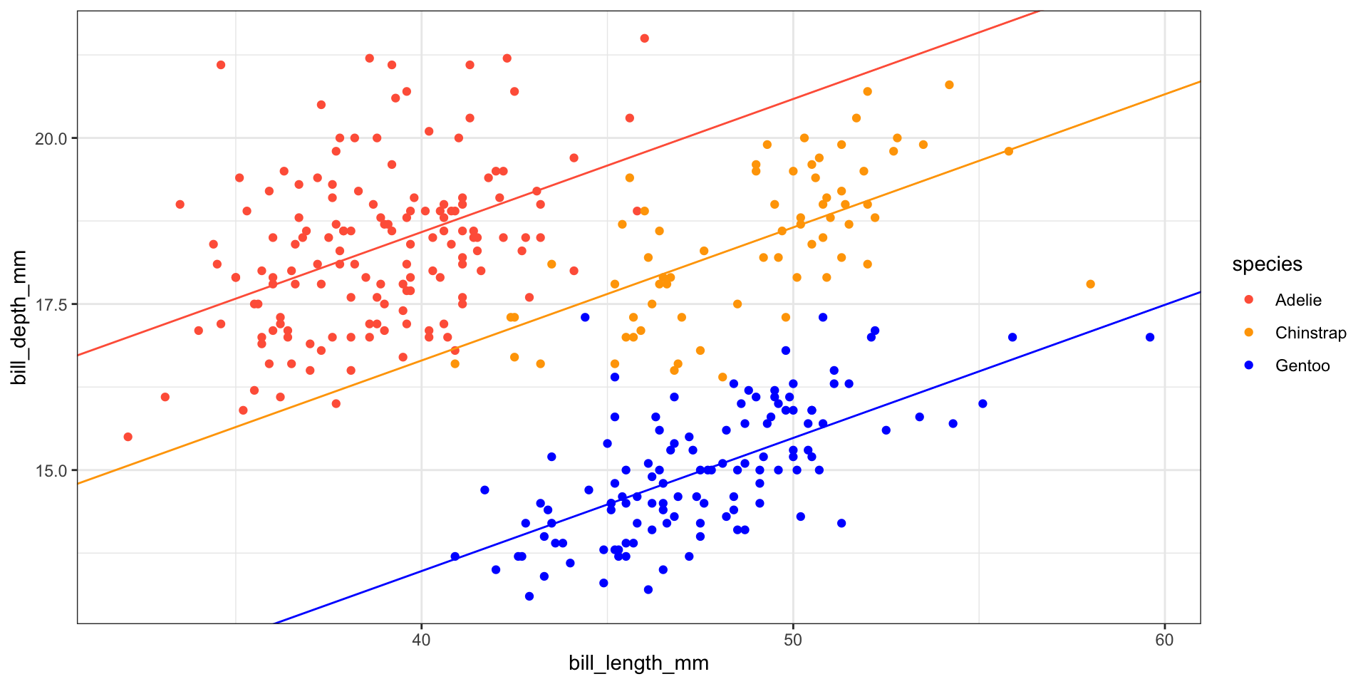
Visualizing lm2 (2 numerical, 1 categorical)

Visualizing lm3 (3 numerical)

tinyurl.com/2hj5x7k3

Practice Problems

25:00

Lab 3.2) Flights

45:00

End of Lecture