[1] 0.3989423Normal Approximation and Box Models
STAT 20: Introduction to Probability and Statistics
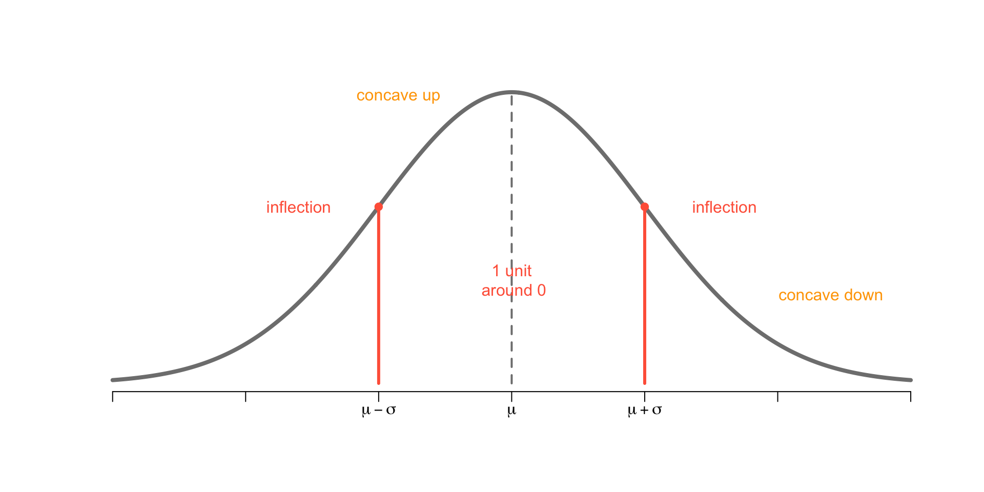
Anatomy of Normal Curve
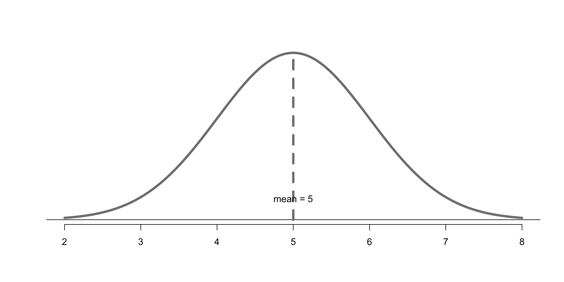
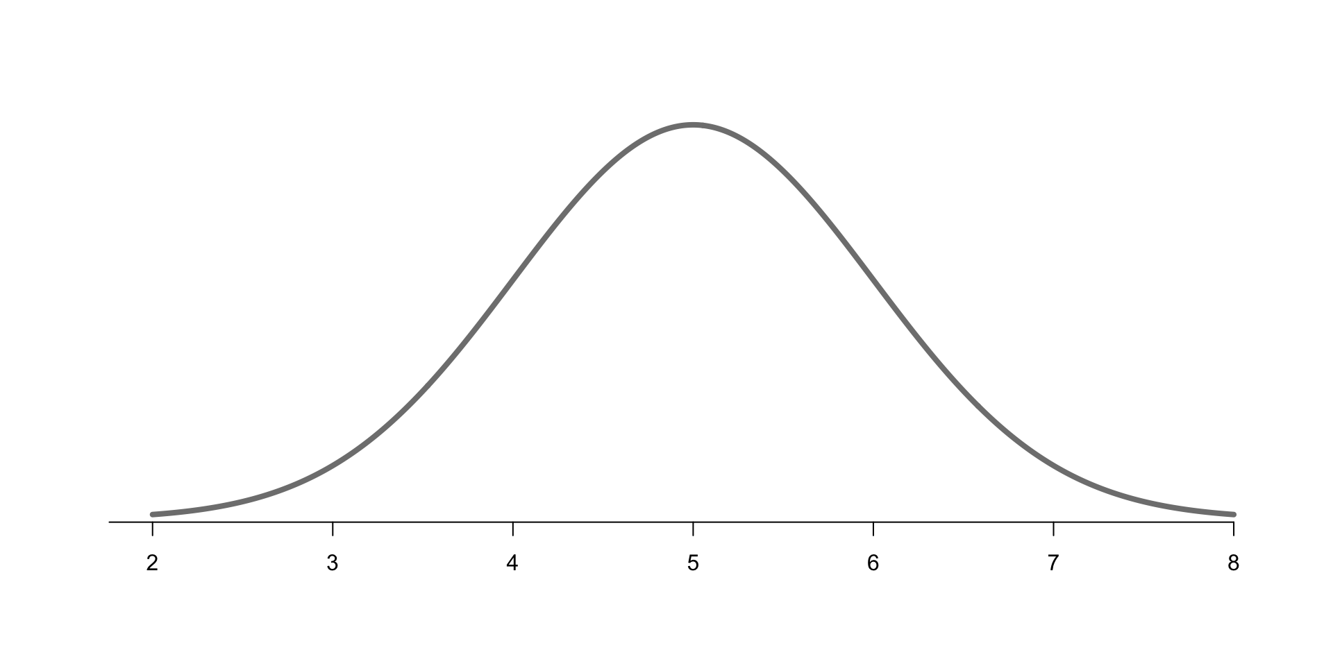
Normal Distribution: \(\mu = 5\), \(\sigma=1\)
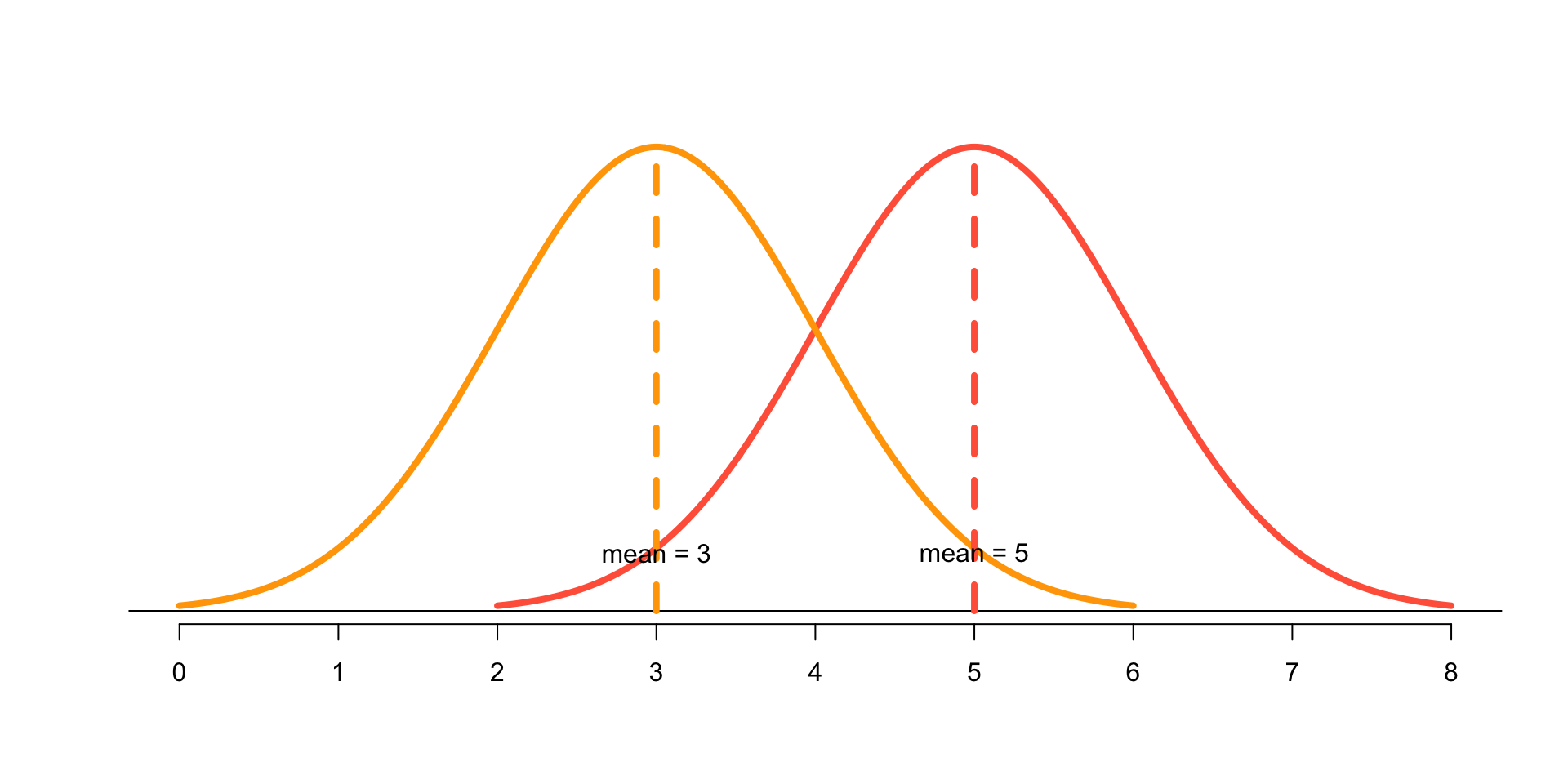
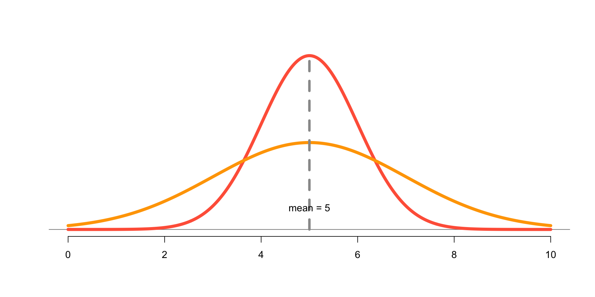
Normal Distributions: different means
Normal Distributions: different std-devs
Normal Distribution
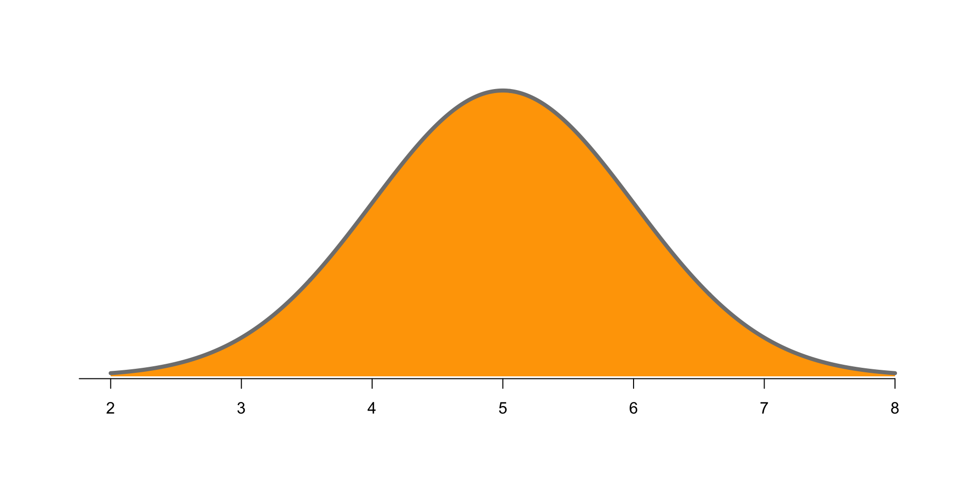
Total area under the curve?
Normal Distribution
Total area under the curve is 1
68% of area within \(1 \sigma\)
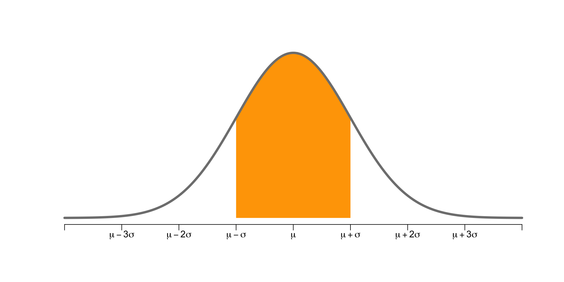
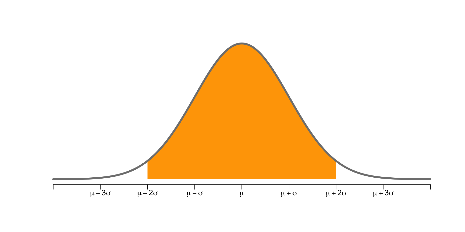
95% of area within \(2 \sigma\)
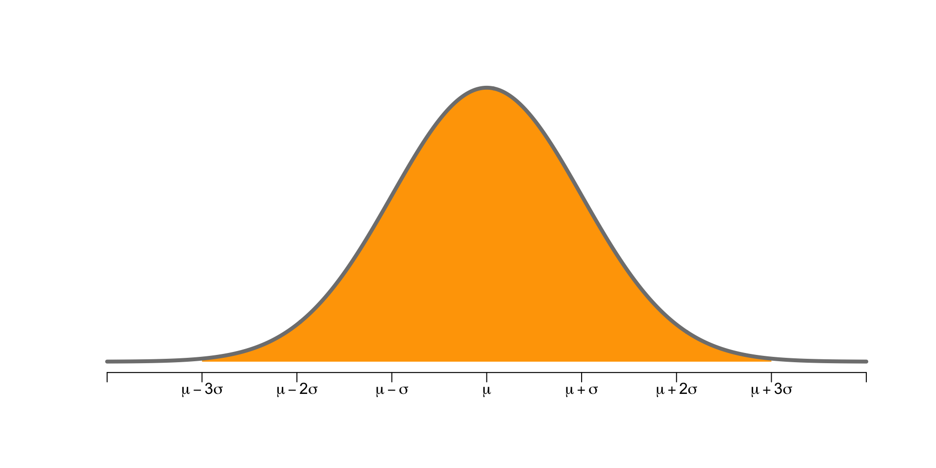
99.7% of area within \(3 \sigma\)
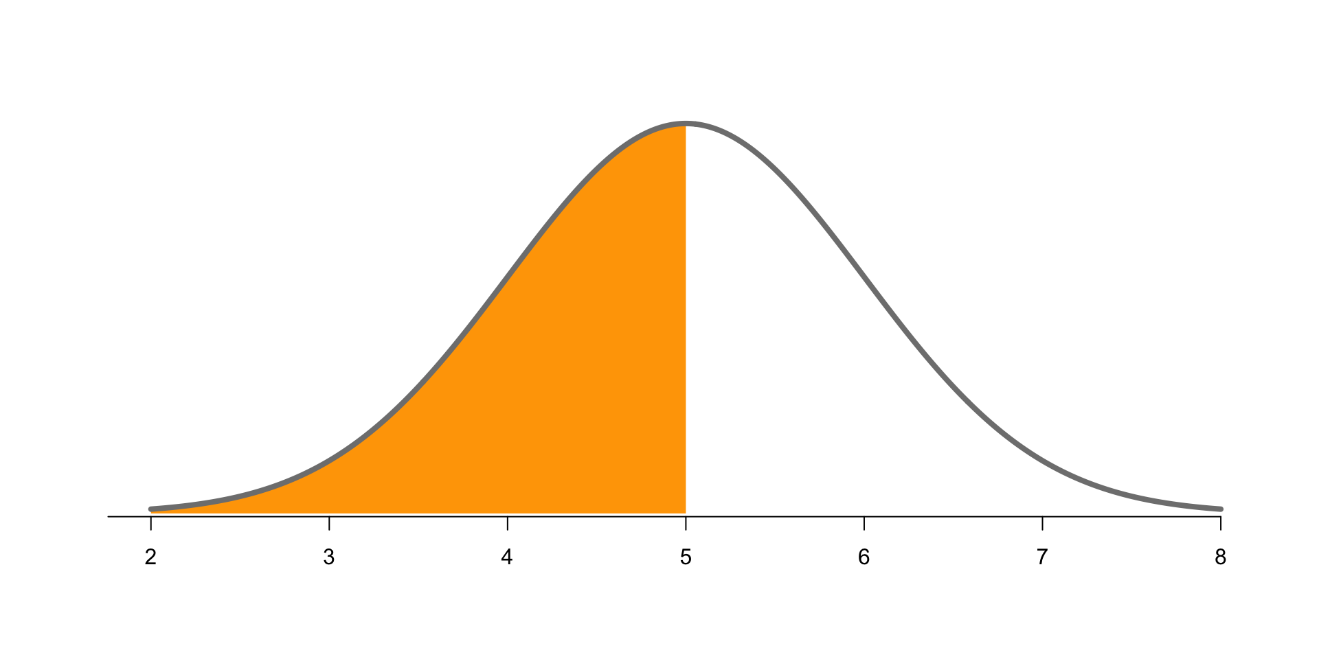
\(P(X \leq 5)\) for \(X \sim N(\mu = 5, \sigma=1)\)
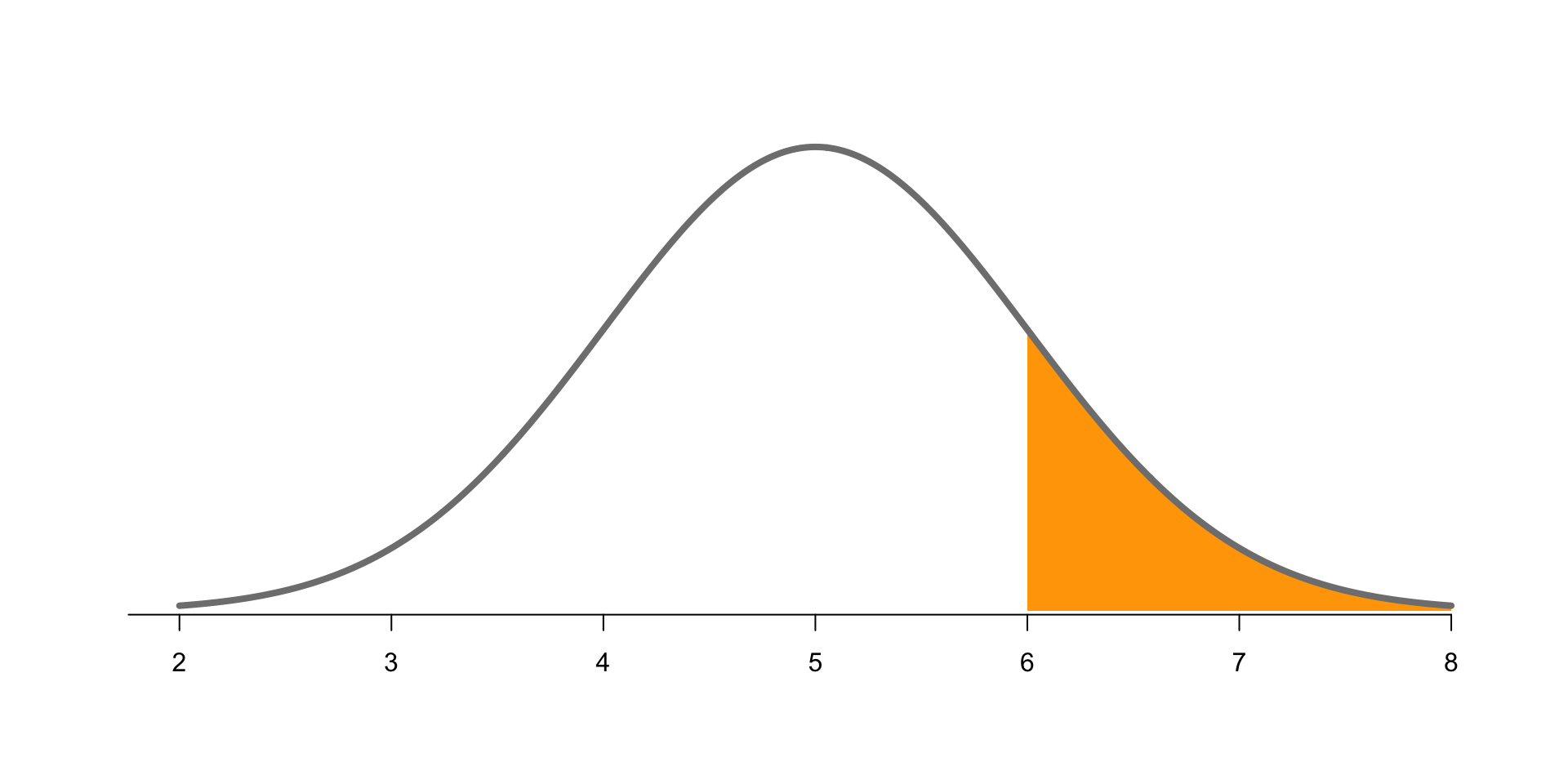
\(P(X \geq 6)\) for \(X \sim N(\mu = 5, \sigma=1)\)
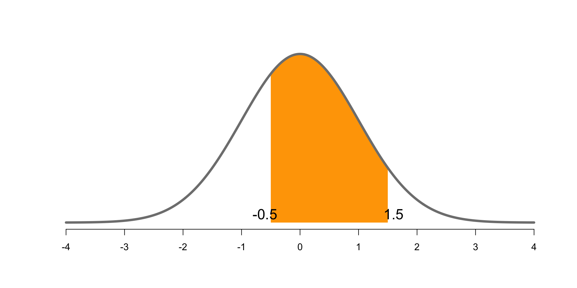
\(P(-0.5 \leq X \leq 1.5)\) for \(X \sim N(\mu = 0, \sigma=1)\)
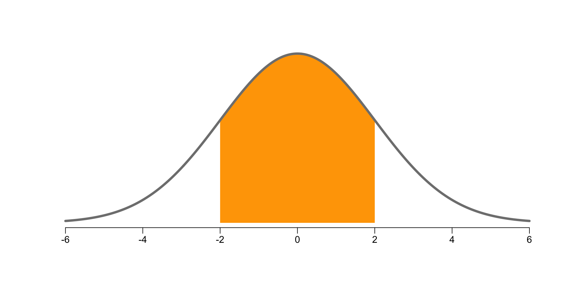
\(P(-2 \leq X \leq 2)\) for \(X \sim N(\mu = 0, \sigma=2)\)
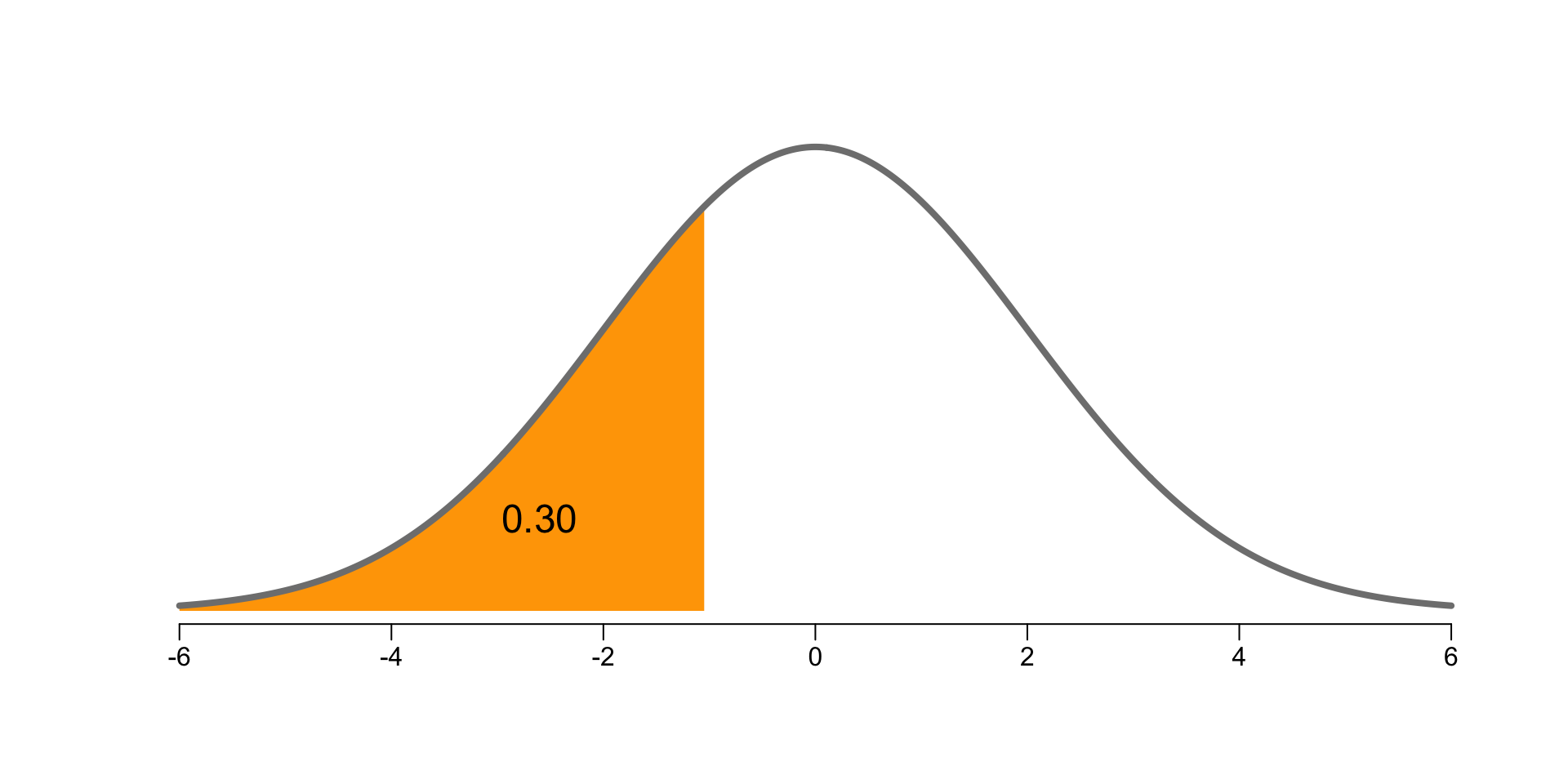
\(P(X \leq x) = 0.3\) for \(X \sim N(\mu = 0, \sigma=2)\)
Example: American Roulette
Code
gains <- replicate(
  n = 1000, # 1000 repetitions
  expr = {
    # net gain in 10 spins of roulette
    spins = sample(x = gain, size = 10, prob = prob_gain, replace = TRUE)
    gain = sum(spins)
})

# empirical histogram
data.frame(gains) |>
  ggplot(aes(x = gains)) +
  geom_histogram(color = "white", binwidth = 2) +
  labs(title = "N = 10",
       x = "net gain") +
  theme_bw()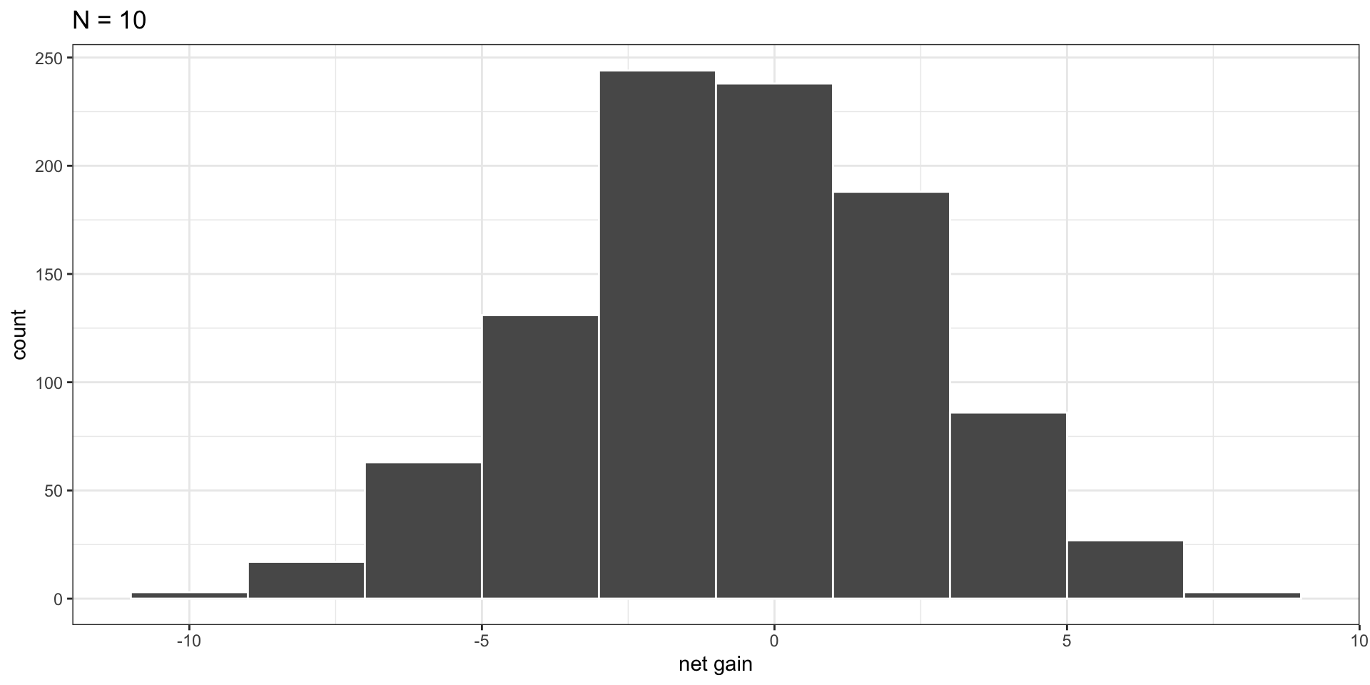
Code
gains <- replicate(
  n = 1000, # 1000 repetitions
  expr = {
    # net gain in 10 spins of roulette
    spins = sample(x = gain, size = 100, prob = prob_gain, replace = TRUE)
    gain = sum(spins)
})

# empirical histogram
data.frame(gains) |>
  ggplot(aes(x = gains)) +
  geom_histogram(color = "white", binwidth = 2) +
  labs(title = "N = 100",
       x = "net gain") +
  theme_bw()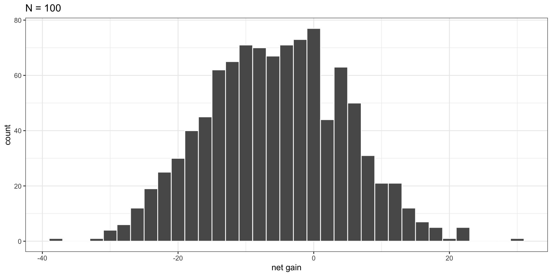
Code
gains <- replicate(
  n = 1000, # 1000 repetitions
  expr = {
    # net gain in 10 spins of roulette
    spins = sample(x = gain, size = 1000, prob = prob_gain, replace = TRUE)
    gain = sum(spins)
})

# empirical histogram
data.frame(gains) |>
  ggplot(aes(x = gains)) +
  geom_histogram(color = "white", binwidth = 8) +
  labs(title = "N = 1000",
       x = "net gain") +
  theme_bw()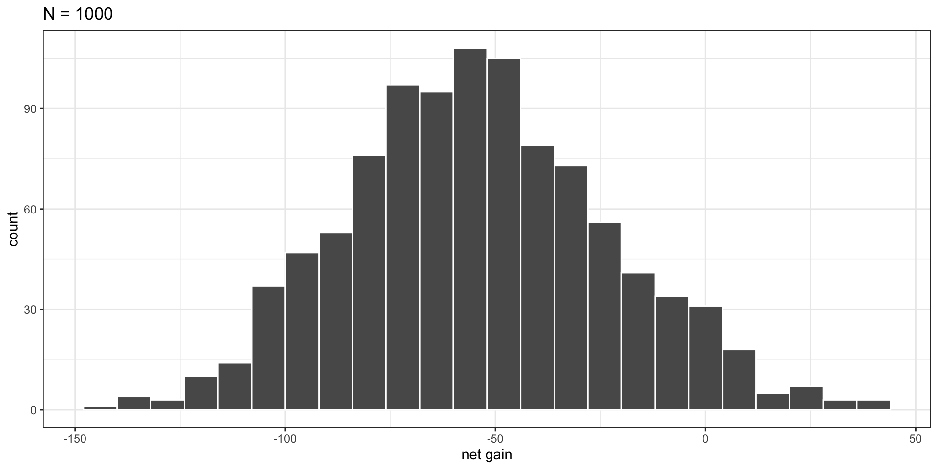
Code
gains <- replicate(
n = 1000, # 1000 repetitions
expr = {
# net gain in 10 spins of roulette
spins = sample(x = gain, size = 5000, prob = prob_gain, replace = TRUE)
gain = sum(spins)
})
# empirical histogram
data.frame(gains) |>
ggplot(aes(x = gains)) +
geom_histogram(color = "white", binwidth = 15) +
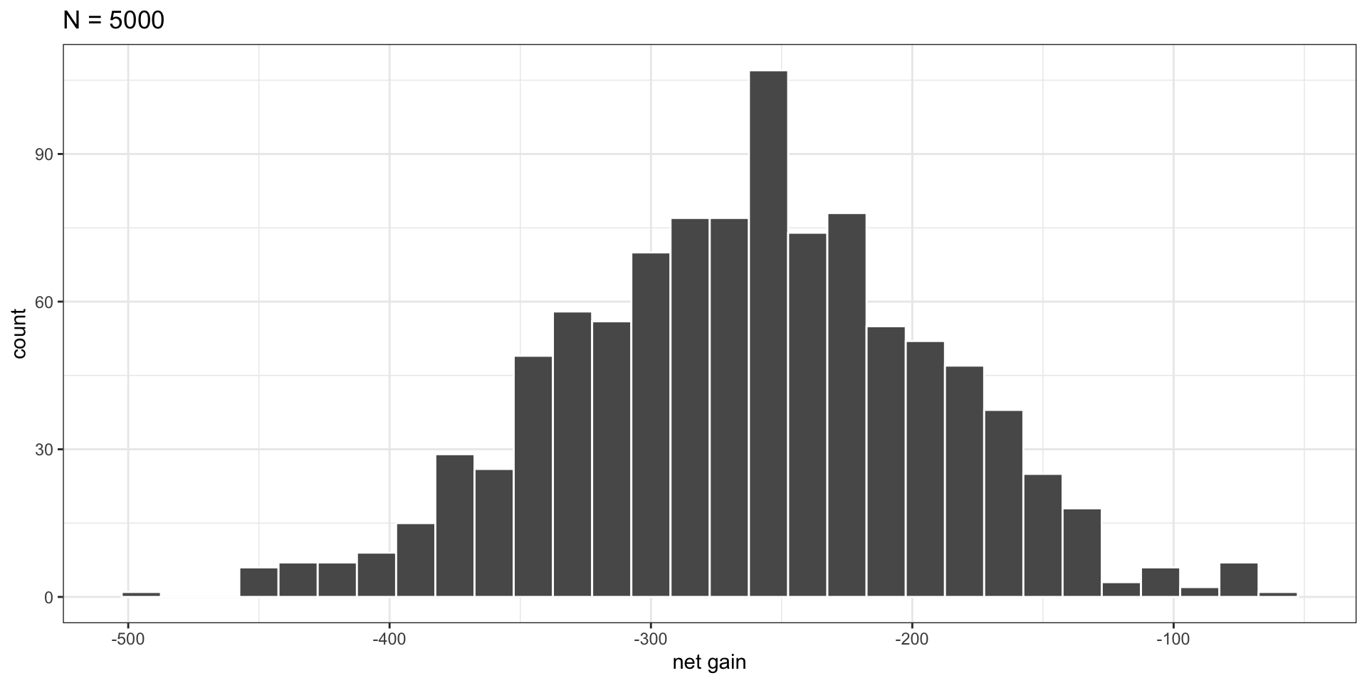
labs(title = "N = 5000",
x = "net gain") +
theme_bw()