6 ways of mean-centering data in R

Posted on January 15, 2014

One of the most frequent operations in multivariate data analysis is the so-called mean-centering. In this post, I’ll show you six different ways to mean-center your data in R.

Mean-centering

Prior to the application of many multivariate methods, data are often pre-processed. This pre-processing involves transforming the data into a suitable form for the analysis. Among the different pre-treatment procedures, one of the most common operations is the well known mean-centering.

Mean-centering involves the subtraction of the variable averages from the data. Since multivariate data is typically handled in table format (i.e. matrix) with columns as variables, mean-centering is often referred to as column centering.

What we do with mean-centering is to calculate the average value of each variable and then subtract it from the data. This implies that each column will be transformed in such a way that the resulting variable will have a zero mean.

Algebraic standpoint

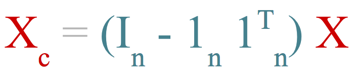
Algebraically, data-centering can be seen as a transformation. This transformation is done using what we could name as a matrix-centering operator denoted by \( H \)

where \( I \) is the identity matrix of size \( n \), \( 1 \) is a vector of ones of length \(n\), and \( n \) is the number of rows in the data \(X\). If we premultiply \(X\) by \(H\) we get the centered matrix \(X_c\):

Equivalently, if we denote by \( \bar{x} \) the vector of column-averages, the mean-centered matrix can be calculated as:

From a geometric point of view, data-centering is just a traslation or repositioning of the coordinate system. In other words, the mean-centering procedure corresponds to moving the origin of the coordinate system to coincide with the average point.

Mean-cenetring in R

Data can be mean-centered in R in several ways, and you can even write your own mean-centering function. I’ll discuss six different ways to do it. More interestingly, we’ll compare those six options to see which one is the fastest.

For illustration purposes we’ll use the following random small dataset:

# small dataset
set.seed(212)
Data = matrix(rnorm(15), 5, 3)

Data

##         [,1]    [,2]    [,3]
## [1,] -0.2392  0.1545  0.1503
## [2,]  0.6769  1.0369  0.5097
## [3,] -2.4403 -0.7796 -0.7733
## [4,]  1.2409  0.6213  1.8757
## [5,] -0.3265  0.2994  0.7883

Using the scale function

Perhaps the most simple, quick and direct way to mean-center your data is by using the function scale(). By default, this function will standardize the data (mean zero, unit variance). To indicate that we just want to subtract the mean, we need to turn off the argument scale = FALSE.

# centering with 'scale()'
center_scale <- function(x) {
    scale(x, scale = FALSE)
}

# apply it
center_scale(Data)

##          [,1]     [,2]       [,3]
## [1,] -0.02153 -0.11200 -0.3597876
## [2,]  0.89458  0.77038 -0.0004599
## [3,] -2.22270 -1.04610 -1.2834512
## [4,]  1.45853  0.35477  1.3655295
## [5,] -0.10887  0.03294  0.2781693
## attr(,"scaled:center")
## [1] -0.2176  0.2665  0.5101

Using the apply function

Center can be done with the apply() function. In this case, the idea is to remove the mean on each column. This is done by declaring a function (inside apply()) that performs the mean-centering operation:

# center with 'apply()'
center_apply <- function(x) {
    apply(x, 2, function(y) y - mean(y))
}

# apply it
center_apply(Data)

##          [,1]     [,2]       [,3]
## [1,] -0.02153 -0.11200 -0.3597876
## [2,]  0.89458  0.77038 -0.0004599
## [3,] -2.22270 -1.04610 -1.2834512
## [4,]  1.45853  0.35477  1.3655295
## [5,] -0.10887  0.03294  0.2781693

Using the sweep function

Another interesting option to mean-center our data is by using the function sweep(). This function has some similarities with apply(). If you give sweep() a value (i.e. a summary statistic) and a function, it will sweep it out on the indicated margin (either by rows or by columns). In our case, the statistic to sweep out by columns is the mean of every variable.

# center with 'sweep()'
center_sweep <- function(x, row.w = rep(1, nrow(x))/nrow(x)) {
    get_average <- function(v) sum(v * row.w)/sum(row.w)
    average <- apply(x, 2, get_average)
    sweep(x, 2, average)
}

# apply it
center_sweep(Data)

##          [,1]     [,2]       [,3]
## [1,] -0.02153 -0.11200 -0.3597876
## [2,]  0.89458  0.77038 -0.0004599
## [3,] -2.22270 -1.04610 -1.2834512
## [4,]  1.45853  0.35477  1.3655295
## [5,] -0.10887  0.03294  0.2781693

Using the colMeans function

Other function that we can take advantage of colMeans(). With this function we can calculate the average value of each column; then we can construct a matrix with the averages, which will be subtracted from the data:

# center with 'colMeans()'
center_colmeans <- function(x) {
    xcenter = colMeans(x)
    x - rep(xcenter, rep.int(nrow(x), ncol(x)))
}

# apply it
center_colmeans(Data)

##          [,1]     [,2]       [,3]
## [1,] -0.02153 -0.11200 -0.3597876
## [2,]  0.89458  0.77038 -0.0004599
## [3,] -2.22270 -1.04610 -1.2834512
## [4,]  1.45853  0.35477  1.3655295
## [5,] -0.10887  0.03294  0.2781693

Using a center-operator

We can create the mean-center operator \(H\) and use it to premultiply the data matrix like so:

# center matrix operator
center_operator <- function(x) {
    n = nrow(x)
    ones = rep(1, n)
    H = diag(n) - (1/n) * (ones %*% t(ones))
    H %*% x
}

# apply it
center_operator(Data)

##          [,1]     [,2]       [,3]
## [1,] -0.02153 -0.11200 -0.3597876
## [2,]  0.89458  0.77038 -0.0004599
## [3,] -2.22270 -1.04610 -1.2834512
## [4,]  1.45853  0.35477  1.3655295
## [5,] -0.10887  0.03294  0.2781693

Using mean subtraction

Finally, we can write a function that implements the algebraic alternative in which the mean-vector is used to create the mean-matrix that is subtracted from the data:

# mean subtraction
center_mean <- function(x) {
    ones = rep(1, nrow(x))
    x_mean = ones %*% t(colMeans(x))
    x - x_mean
}

# apply it
center_mean(Data)

##          [,1]     [,2]       [,3]
## [1,] -0.02153 -0.11200 -0.3597876
## [2,]  0.89458  0.77038 -0.0004599
## [3,] -2.22270 -1.04610 -1.2834512
## [4,]  1.45853  0.35477  1.3655295
## [5,] -0.10887  0.03294  0.2781693

What option to use?

So far we’ve seen six different ways in which we can mean-center a matrix. But what option is the more efficient (computationally)? To get an answer nothing better than make a small contest to see which of our 6 options is the fastest (and which one the slowest):

# fake data
X = matrix(runif(2000), 100, 20)

# test them
system.time(replicate(500, center_scale(X)))

##    user  system elapsed 
##   0.106   0.004   0.110

system.time(replicate(500, center_apply(X)))

##    user  system elapsed 
##   0.239   0.009   0.248

system.time(replicate(500, center_sweep(X)))

##    user  system elapsed 
##   0.222   0.010   0.232

system.time(replicate(500, center_colmeans(X)))

##    user  system elapsed 
##   0.060   0.000   0.061

system.time(replicate(500, center_operator(X)))

##    user  system elapsed 
##   0.209   0.037   0.244

system.time(replicate(500, center_mean(X)))

##    user  system elapsed 
##   0.066   0.001   0.067

And the winner is … center_colmeans()