5 functions to do Correspondence Analysis in R
Posted on July 19, 2012
In a previous post, I talked about five different ways to do Principal Components Analysis in R
PCA is very useful and is one of the most applied multivariate techniques. However, PCA is limited to quantitative information. But what if our data comes in the form of qualitative information such as categorical data? The solution: Correspondence Analysis.
Correspondence Analysis, briefly CA, is one of the cousins of Principal Component Analysis. Both CA and PCA are multivariate techniques that help us to summarize the systematic patterns of variations in the data. The difference between CA and PCA is that CA applies to categorical (i.e. qualitative) data instead of continuous (i.e. quantitative) data. More specifically, CA applies to categorical data in the form of contingency tables (aka cross-tabulation). Since CA is conceptually similar to PCA, we can use it, among other things, for visualizing multidimensional data into a lower dimensional space.
CA in R
In R, there are several functions from different packages that allow us to apply Correspondence Analysis. In this post I’ll show you 5 different ways to perform CA using the following functions (with their corresponding packages in parentheses):
ca()(ca)CA()(FactoMineR)dudi.coa()(ade4)afc()(amap)corresp()(MASS)
As in PCA, no matter what function you decide to use for CA, the typical results should consist of a set of eigenvalues, a table with the row coordinates, and a table with the column coordinates. The eigenvalues provide information of the variability in the data. The row coordinates provide information about the structure of the rows in the analyzed table. The column coordinates provide information about the structure of the columns in the analyzed table.
The Data
We’ll use the dataset author that already comes with the R package "ca". It’s a data matrix containing the counts of the 26 letters of the alphabet (columns of matrix) for 12 different novels (rows of matrix). Each row contains letter counts in a sample of text from each work, excluding proper nouns.
Option 1: using ca
The function ca() comes in the package of the same name ca by Michael Greenacre and Oleg Nenadic. I personally like this package because of Greenacre’s work and books about CA. In addition, it has a very nice function to plot results in 3D (plot3d.ca())
# CA with function ca
library(ca)

# apply ca
ca1 = ca(author)

# sqrt of eigenvalues
ca1$sv
## [1] 0.08754 0.06073 0.04910 0.03719 0.03165 0.02689 0.02566 0.02133
## [9] 0.01934 0.01622 0.01064# row coordinates
head(ca1$rowcoord)## [,1] [,2] [,3] [,4] [,5] [,6] [,7] [,8]
## [1,] -0.09539 -0.79500 1.0285 0.6472 1.13597 -0.3149 -0.9908 0.7942
## [2,] 0.40570 -0.40556 -0.9304 0.6344 -0.08487 -1.7388 -1.0871 0.9097
## [3,] 1.15780 -0.02311 0.3551 1.0639 -1.33880 1.0157 0.3715 1.3790
## [4,] -0.17390 0.43444 2.0871 -0.2991 0.96081 -0.5655 0.3561 0.3814
## [5,] -0.83189 -0.13648 -0.9437 1.2758 1.11671 2.2559 -0.2008 -0.1684
## [6,] 0.30203 2.70760 -0.1815 0.7055 0.30494 -0.4697 -0.3644 -1.3977
## [,9] [,10] [,11]
## [1,] -1.64567 1.6411 0.4328
## [2,] -0.36151 -1.8976 -1.0833
## [3,] 1.15739 0.9237 -1.0610
## [4,] 1.53050 -1.0166 0.7930
## [5,] 0.03299 -1.1202 0.5232
## [6,] -0.20322 0.6567 -0.5689# column coordinates
head(ca1$colcoord)## [,1] [,2] [,3] [,4] [,5] [,6] [,7] [,8]
## [1,] 0.01762 -0.3203 -0.2704 0.6478 -0.4436 0.7176 0.27348 -1.09591
## [2,] 0.98446 -0.3980 1.1490 -1.6202 -0.4042 -1.8570 -1.88405 -1.70703
## [3,] 2.11503 -1.3734 -1.1309 -0.9539 -1.0867 -0.2066 0.57144 -2.03364
## [4,] -1.92563 -1.1354 0.2934 -0.2390 -0.1604 -0.5917 0.41892 1.52674
## [5,] 0.08672 -0.6848 1.0038 0.3656 -0.1529 0.3979 0.07591 0.37646
## [6,] 1.27653 -0.7330 -0.3865 -0.4409 1.5577 -3.0251 0.28235 -0.01798
## [,9] [,10] [,11]
## [1,] 0.3149 0.1593 0.05681
## [2,] 1.0259 0.8911 -1.32001
## [3,] -1.2373 -0.5709 -0.84705
## [4,] -1.6798 -0.1750 -0.93757
## [5,] -1.0090 -0.1227 0.40216
## [6,] 1.6629 -2.2692 -2.62764# plot
plot(ca1)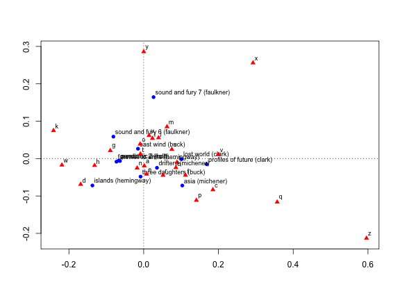
Option 2: using CA
One of my favorite options is the CA() function from the packageFactoMineR. What I like is that this function provides many more detailed results and assessing tools. It also comes with a number of parameters that allow you to tweak the analysis in a very nice way.
# CA with function CA
library(FactoMineR)

# apply CA
ca2 = CA(author, graph = FALSE)

# matrix with eigenvalues
ca2$eig
## eigenvalue percentage of variance cumulative percentage of variance
## dim 1 0.0076639 40.9070 40.91
## dim 2 0.0036883 19.6870 60.59
## dim 3 0.0024112 12.8702 73.46
## dim 4 0.0013828 7.3811 80.85
## dim 5 0.0010017 5.3465 86.19
## dim 6 0.0007233 3.8609 90.05
## dim 7 0.0006586 3.5154 93.57
## dim 8 0.0004548 2.4278 96.00
## dim 9 0.0003739 1.9958 97.99
## dim 10 0.0002631 1.4041 99.40
## dim 11 0.0001132 0.6042 100.00# row coordinates
head(ca2$col$coord)## Dim 1 Dim 2 Dim 3 Dim 4 Dim 5
## a 0.001543 -0.01945 0.01328 -0.024088 0.014040
## b 0.086183 -0.02417 -0.05642 0.060250 0.012792
## c 0.185157 -0.08341 0.05553 0.035473 0.034392
## d -0.168576 -0.06895 -0.01441 0.008886 0.005076
## e 0.007592 -0.04159 -0.04929 -0.013595 0.004841
## f 0.111752 -0.04451 0.01898 0.016396 -0.049299# column coordinates
head(ca2$row$coord)## Dim 1 Dim 2 Dim 3 Dim 4
## three daughters (buck) -0.008351 -0.048282 -0.050505 -0.02407
## drifters (michener) 0.035516 -0.024630 0.045687 -0.02359
## lost world (clark) 0.101358 -0.001404 -0.017436 -0.03956
## east wind (buck) -0.015224 0.026384 -0.102483 0.01112
## farewell to arms (hemingway) -0.072826 -0.008289 0.046339 -0.04744
## sound and fury 7 (faulkner) 0.026440 0.164437 0.008911 -0.02624
## Dim 5
## three daughters (buck) -0.035952
## drifters (michener) 0.002686
## lost world (clark) 0.042372
## east wind (buck) -0.030409
## farewell to arms (hemingway) -0.035343
## sound and fury 7 (faulkner) -0.009651# plot
plot(ca2)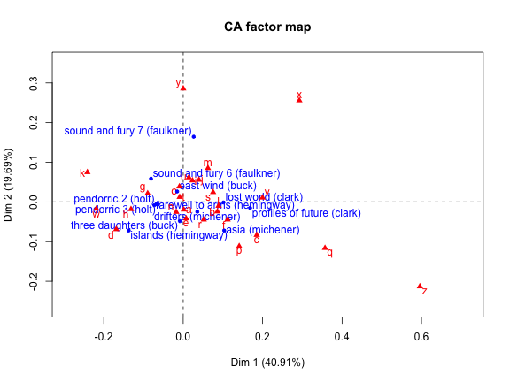
Option 3: using dudi.coa
Another option to perform CA is by using the function dudi.coa()> that comes with the package ade4 (remember to install the package first).
# CA with function dudi.coa
library(ade4)

# apply ca
ca3 = dudi.coa(author, nf = 5, scannf = FALSE)

# sqrt of eigenvalues
ca3$eig
## [1] 0.0076639 0.0036883 0.0024112 0.0013828 0.0010017 0.0007233 0.0006586
## [8] 0.0004548 0.0003739 0.0002631 0.0001132# row coordinates
head(ca3$li)## Axis1 Axis2 Axis3 Axis4
## three daughters (buck) 0.008351 0.048282 0.050505 -0.02407
## drifters (michener) -0.035516 0.024630 -0.045687 -0.02359
## lost world (clark) -0.101358 0.001404 0.017436 -0.03956
## east wind (buck) 0.015224 -0.026384 0.102483 0.01112
## farewell to arms (hemingway) 0.072826 0.008289 -0.046339 -0.04744
## sound and fury 7 (faulkner) -0.026440 -0.164437 -0.008911 -0.02624
## Axis5
## three daughters (buck) -0.035952
## drifters (michener) 0.002686
## lost world (clark) 0.042372
## east wind (buck) -0.030409
## farewell to arms (hemingway) -0.035343
## sound and fury 7 (faulkner) -0.009651# column coordinates
head(ca3$co)## Comp1 Comp2 Comp3 Comp4 Comp5
## a -0.001543 0.01945 -0.01328 -0.024088 0.014040
## b -0.086183 0.02417 0.05642 0.060250 0.012792
## c -0.185157 0.08341 -0.05553 0.035473 0.034392
## d 0.168576 0.06895 0.01441 0.008886 0.005076
## e -0.007592 0.04159 0.04929 -0.013595 0.004841
## f -0.111752 0.04451 -0.01898 0.016396 -0.049299Option 4: using afc
Another option is to use the afc() function from the package amap (remember to install it first).
# PCA with function afc
library(amap)

# apply CA
ca4 = afc(author)

# eigenvalues
ca4$eig
## [1] 1.842e-01 1.346e-01 1.036e-01 8.744e-02 6.207e-02 3.470e-02 3.470e-02
## [8] 2.985e-02 2.985e-02 2.419e-02 1.771e-02 4.288e-03 2.034e-09 4.690e-10
## [15] 4.690e-10 9.408e-10 6.620e-10 6.620e-10 3.303e-10 3.303e-10 7.661e-10
## [22] 3.776e-10 3.776e-10 1.919e-10 1.919e-10 1.337e-10# row coordinates
head(ca4$scores)## Comp 1 Comp 2 Comp 3 Comp 4 Comp 5
## three daughters (buck) 0.4995 0.79652 -0.3461 0.13097 -0.1440
## drifters (michener) -0.2646 -0.80085 -0.1714 0.07223 -0.4803
## lost world (clark) -1.3028 -0.53461 -0.3125 0.22787 -0.3724
## east wind (buck) 0.4863 0.02159 -0.4983 0.01119 -0.2621
## farewell to arms (hemingway) 1.3600 0.59080 0.4792 0.46053 0.4875
## sound and fury 7 (faulkner) 0.9175 -0.36445 -0.9206 0.65150 0.2866
## Comp 6 Comp 7 Comp 8 Comp 9 Comp 10
## three daughters (buck) -0.01648 -0.01648 0.07180 0.07180 -0.22287
## drifters (michener) 0.19286 0.19286 -0.18403 -0.18403 0.24843
## lost world (clark) -0.12196 -0.12196 0.14200 0.14200 -0.18316
## east wind (buck) -0.32069 -0.32069 0.35655 0.35655 -0.33860
## farewell to arms (hemingway) -0.05868 -0.05868 0.06305 0.06305 -0.11130
## sound and fury 7 (faulkner) -0.27843 -0.27843 0.14867 0.14867 -0.07467
## Comp 11 Comp 12 Comp 13 Comp 14 Comp 15
## three daughters (buck) -0.17961 -0.03171 -0.14867 0.01262 0.01262
## drifters (michener) 0.11556 0.11611 -0.04248 -0.09915 -0.09915
## lost world (clark) -0.09069 0.09037 0.14241 0.10192 0.10192
## east wind (buck) -0.38149 -0.13807 -0.22816 0.03239 0.03239
## farewell to arms (hemingway) -0.09531 -0.08273 -0.06196 0.01321 0.01321
## sound and fury 7 (faulkner) 0.02458 0.21285 0.28994 0.02993 0.02993
## Comp 16 Comp 17 Comp 18 Comp 19
## three daughters (buck) -0.04379 -0.062066 -0.062066 0.07056
## drifters (michener) -0.27515 -0.055491 -0.055491 0.10012
## lost world (clark) 0.02816 0.074598 0.074598 -0.09971
## east wind (buck) 0.03484 0.004923 0.004923 0.02259
## farewell to arms (hemingway) -0.05800 0.020237 0.020237 -0.01491
## sound and fury 7 (faulkner) 0.10525 0.136355 0.136355 -0.14655
## Comp 20 Comp 21 Comp 22 Comp 23 Comp 24
## three daughters (buck) 0.07056 0.048720 0.10302 0.10302 0.07405
## drifters (michener) 0.10012 -0.071811 0.10479 0.10479 0.09259
## lost world (clark) -0.09971 -0.011493 -0.03282 -0.03282 -0.02379
## east wind (buck) 0.02259 0.006737 0.06182 0.06182 0.05335
## farewell to arms (hemingway) -0.01491 -0.046687 0.02372 0.02372 -0.01116
## sound and fury 7 (faulkner) -0.14655 -0.002282 -0.14921 -0.14921 -0.04634
## Comp 25 Comp 26
## three daughters (buck) 0.07405 -0.06265
## drifters (michener) 0.09259 -0.07276
## lost world (clark) -0.02379 -0.05611
## east wind (buck) 0.05335 -0.06700
## farewell to arms (hemingway) -0.01116 -0.03241
## sound and fury 7 (faulkner) -0.04634 0.03541# column coordinates
head(ca4$loadings)## Comp 1 Comp 2 Comp 3 Comp 4 Comp 5 Comp 6 Comp 7
## a 0.003022 0.020612 0.061492 0.06195 0.05277 0.043411 0.043411
## b -0.092480 0.008901 -0.091345 -0.07467 -0.08660 -0.022569 -0.022569
## c -0.178710 0.055824 0.098704 0.13198 0.15376 0.064302 0.064302
## d 0.073138 0.003039 0.156074 -0.34174 -0.29959 0.269560 0.269560
## e -0.019221 0.012044 -0.002028 -0.02439 -0.18621 0.007124 0.007124
## f -0.106717 0.055966 -0.071859 0.04725 -0.06634 -0.096594 -0.096594
## Comp 8 Comp 9 Comp 10 Comp 11 Comp 12 Comp 13 Comp 14 Comp 15
## a -0.06499 -0.06499 0.07583 0.06867 -0.09411 0.20568 0.4721 0.4721
## b -0.03962 -0.03962 0.08500 0.10156 0.28316 -0.03667 -0.2147 -0.2147
## c -0.15066 -0.15066 0.26830 0.40201 -0.01905 0.35904 0.1227 0.1227
## d -0.19360 -0.19360 0.08525 0.15203 0.26842 0.03422 -0.2050 -0.2050
## e 0.04881 0.04881 -0.17418 -0.11241 -0.13982 -0.07567 0.1211 0.1211
## f 0.07174 0.07174 0.19381 0.06160 0.28309 0.02290 -0.1100 -0.1100
## Comp 16 Comp 17 Comp 18 Comp 19 Comp 20 Comp 21 Comp 22 Comp 23
## a -0.28537 0.2721 0.2721 -0.4497 -0.4497 -0.76831 -0.4205 -0.4205
## b 0.11343 -0.1243 -0.1243 0.1913 0.1913 0.22611 0.1029 0.1029
## c 0.01782 0.1082 0.1082 -0.1314 -0.1314 -0.01929 -0.0811 -0.0811
## d -0.34191 -0.3789 -0.3789 0.3926 0.3926 0.11445 0.2280 0.2280
## e -0.07271 0.1265 0.1265 -0.1754 -0.1754 -0.06055 -0.1862 -0.1862
## f -0.38806 -0.2324 -0.2324 0.2252 0.2252 0.04042 0.2155 0.2155
## Comp 24 Comp 25 Comp 26
## a -0.17789 -0.17789 0.24034
## b 0.01092 0.01092 -0.07016
## c -0.01783 -0.01783 0.11984
## d -0.03367 -0.03367 -0.17324
## e -0.04367 -0.04367 0.09777
## f 0.15196 0.15196 -0.16994# plot
plot(ca4)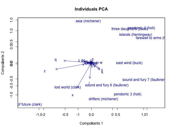
Option 5: using corresp
A fifth possibility is the corresp() function from the package MASS.
# CA with function corresp
library(MASS)

# apply CA
ca5 = corresp(author, nf = 5)

# sqrt of eigenvalues
ca5$cor
## [1] 0.08754 0.06073 0.04910 0.03719 0.03165# row coordinates
head(ca5$rscore)## [,1] [,2] [,3] [,4] [,5]
## three daughters (buck) -0.09539 -0.79500 1.0285 0.6472 1.13597
## drifters (michener) 0.40570 -0.40556 -0.9304 0.6344 -0.08487
## lost world (clark) 1.15780 -0.02311 0.3551 1.0639 -1.33880
## east wind (buck) -0.17390 0.43444 2.0871 -0.2991 0.96081
## farewell to arms (hemingway) -0.83189 -0.13648 -0.9437 1.2758 1.11671
## sound and fury 7 (faulkner) 0.30203 2.70760 -0.1815 0.7055 0.30494# column coordinates
head(ca5$cscore)## [,1] [,2] [,3] [,4] [,5]
## a 0.01762 -0.3203 -0.2704 0.6478 -0.4436
## b 0.98446 -0.3980 1.1490 -1.6202 -0.4042
## c 2.11503 -1.3734 -1.1309 -0.9539 -1.0867
## d -1.92563 -1.1354 0.2934 -0.2390 -0.1604
## e 0.08672 -0.6848 1.0038 0.3656 -0.1529
## f 1.27653 -0.7330 -0.3865 -0.4409 1.5577# plot
plot(ca5)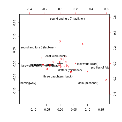
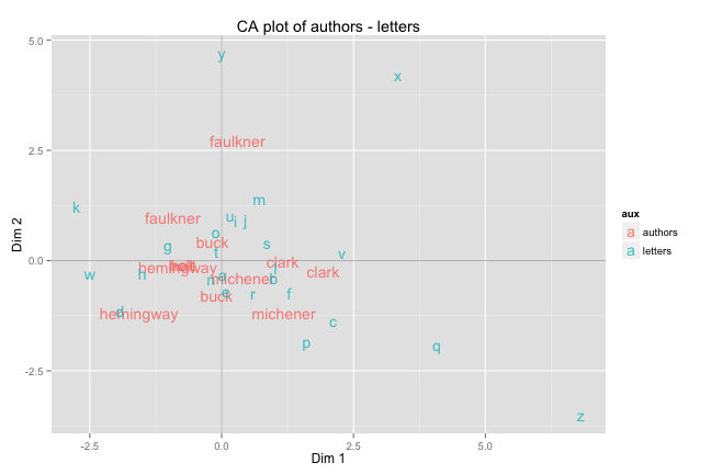
CA plot
The typical graphic in a CA analysis is to visualize the data in a two dimensional space using the first two extracted coordinates from both rows and columns. Although we could visualize the rows and the columns separately, the usual approach is to plot both in a single graphic to get an idea of the association between them. As you can tell from the displayed code chunks, most of the CA functions have their own plot command. However, we can also use the nice tools of "ggplot2". In the following example we will also use the package "stringr"
# load ggplot2
library(ggplot2)
library(stringr)

# extract only author names
authors = rownames(author)
authors = unlist(str_extract_all(authors, "\\(\\w+"))
authors = gsub("\\(", "", authors)

# create data frame with row and col coordinates
# from both the authors and the letters
aux = c(rep("authors", 12), rep("letters", 26))
name = c(authors, colnames(author))
auth_lets = data.frame(
  name, aux, rbind(ca1$rowcoord[,1:2], ca1$colcoord[,1:2]))
head(auth_lets)
## name aux X1 X2
## 1 buck authors -0.09539 -0.79500
## 2 michener authors 0.40570 -0.40556
## 3 clark authors 1.15780 -0.02311
## 4 buck authors -0.17390 0.43444
## 5 hemingway authors -0.83189 -0.13648
## 6 faulkner authors 0.30203 2.70760# plot of authors and letters
ggplot(data = auth_lets, aes(x = X1, y = X2, label = name)) +
geom_hline(yintercept = 0, colour = "gray75") +
geom_vline(xintercept = 0, colour = "gray75") +
geom_text(aes(colour = aux), alpha = 0.8, size = 5) +
labs(x = "Dim 1", y = "Dim 2") +
ggtitle("CA plot of authors - letters")