Column-wise operations with colwise
Posted on February 19, 2013

In a previous post
I described different options in R to do some calculations using tapply(),
ddply(), and sqldf().
I used a simple example in which the goal was to apply a function by groups on some data. More specifically: how to calculate the average of a single variable taking into account a grouping variable (eg categorical variable).
This time I wanted to continue the discussion with another interesting task when operating on grouping variables. Say we have some categorical variable (like gender, geographic region, political affiliation) with other quantitative information. More often than not we want to calculate descriptive statistics taking into account the categorical variable. Maybe we want to calculate the average of all the quantitative variables by gender. How do you do that in R?
There are a number of different options to get the answer. One option is to use the
function colwise() from the package "plyr" (by Hadley Wickham). The idea of
colwise() is to turn a function that operates on a vector into a function that
operates column-wise on a data.frame. The trick is to use colwise() inside
the function ddply(). Here’s a simple example:
# generate some fake data
# (use 'set.seed' for replication purposes)
set.seed(80)
some_data = data.frame(matrix(rnorm(75), nrow=15, ncol=5))

# add categorical variable 'Group' (there will be 5 groups)
some_data$Group = as.factor(paste("Group", rep(1:5, each=3), sep="_"))

# load package plyr
require(plyr)

# ddply with colwise operation
group_means_data = ddply(some_data, .(Group), colwise(mean))

# get group means
group_means = as.matrix(group_means_data[,-1])
rownames(group_means) = group_means_data$Group

# inspect the results
group_means
You should get something like this:
X1 X2 X3 X4 X5
Group_1 0.30145430 0.05948726 -0.4638955 -0.08925132 0.1919387
Group_2 0.10691675 -0.07851064 -0.1248169 -0.32776258 0.5754724
Group_3 -0.23172617 -0.10895998 -0.5388441 0.21742869 0.1327649
Group_4 -0.41673809 0.90000430 -0.5448786 -0.16260781 0.3347490
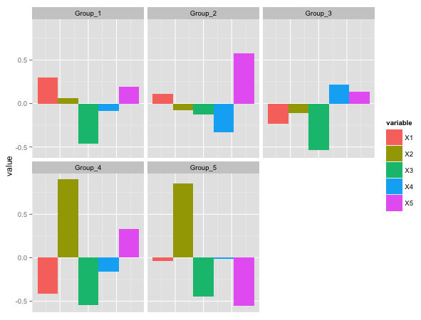
Group_5 -0.03758755 0.85385634 -0.4445546 -0.01103586 -0.5547903We have the average values of all the variables for each group. Now let’s visualize them to have a better idea of what’s going on:
# load 'ggplot2' and 'reshape'
library(ggplot2)
library(reshape)

# melt data
group_means_melt = melt(group_means_data)

# add auxiliar variable (for plotting purposes)
group_means_melt$aux = rep(1, nrow(group_means_melt))

# barplots for each group
ggplot(group_means_melt, aes(x = aux, y = value, fill = variable)) +
  geom_bar(stat = "identity", position = "dodge") +
  facet_wrap(~ Group) +
  xlab("") +
  theme(axis.text.x = element_blank(),
        axis.ticks.x = element_blank())