5 Playing Game-A 100 times

With all the coding elements that we have discussed so far, it’s time to play Game-A 100 times, and see what the proportion of wins turns out to be:

# random seed (for reproducibility purposes)
set.seed(753)

# main inputs
die = 1:6
number_games = 100

# initialize output matrix
games = matrix(0, nrow = number_games, ncol = 4)

# playing Game-A several times
for (game in 1:number_games) {
  games[game, ] = sample(die, size = 4, replace = TRUE)
}

rownames(games) = paste0("game", 1:number_games)
colnames(games) = paste0("roll", 1:4)

# determine each game's win-or-lose output
wins = apply(
  X = games, 
  MARGIN = 1,
  FUN = function(x) any(x == 6))

# total proportion of wins
prop_wins = sum(wins) / number_games
prop_wins

## [1] 0.5

In this particular simulation of 100 games, we end up with a 0.5 proportion of wins. In other words, 50 percent of the games are wins, and the other 50 percent of the games are losses.

5.1 Computing Cumulative Gains

To make things more interesting, let’s assume that you are paid $1 if you win a game, but also that you pay $1 if you lose a game. That is:

• gain 1 if you win a game

• gain -1 if you lose a game

This means that we need to create another object to store this “gains” information. This can be done in different ways. One option is to initialize a vector gains of length number_games, and set its elements to -1. Then use the logical vector wins to do logical subsetting and switch to 1 the elements matching the TRUE values in wins, like this:

# vector of gains
gains = rep(-1, number_games)  # initialize with all -1 elements
gains[wins] = 1                # switch to +1 for every win

The vector gains is a numeric vector containing as many 1’s as wins, and as many -1 as losses:

table(wins)

## wins
## FALSE  TRUE 
##    50    50

More interestingly, we can use cumsum() to obtain the cumulative addition of all elements in wins. The output vector, cumulative_gains, will contain the sequence of cumulative gains along the 100 games.

# cumulative gains
cumulative_gains = cumsum(gains)

head(cumulative_gains, n = 10)

##  [1]  1  2  1  0 -1 -2 -1 -2 -3 -4

As you can tell from this output, the first game is a win, as well as the second one. But then, we get a decreasing sequence with the next four elements in cumulative_gains: 1 0 -1 -2, indicating that games 3 to 6 are consecutive losses.

5.2 Plotting Cumulative Gains

It would be nice to visualize the sequence of wins and losses using the vector of cumulative gains cumulative_gains. So let’s see how to get some plots using base "graphics" functions, as well as "ggplot2" functions.

5.2.1 Cumulative Gains with plot()

Using traditional "graphics" functions, we can create a line graph with plot(). In the x-axis we pass a sequence vector of games; as for the y-axis we pass the cumulative_gains vector.

plot(1:number_games, cumulative_gains, type = 'l',
     xlab = "games", ylab = "cumulative gain", las = 1,
     lwd = 1.5, col = "#318BEC")
abline(h = 0, col = "gray70", lty = 2)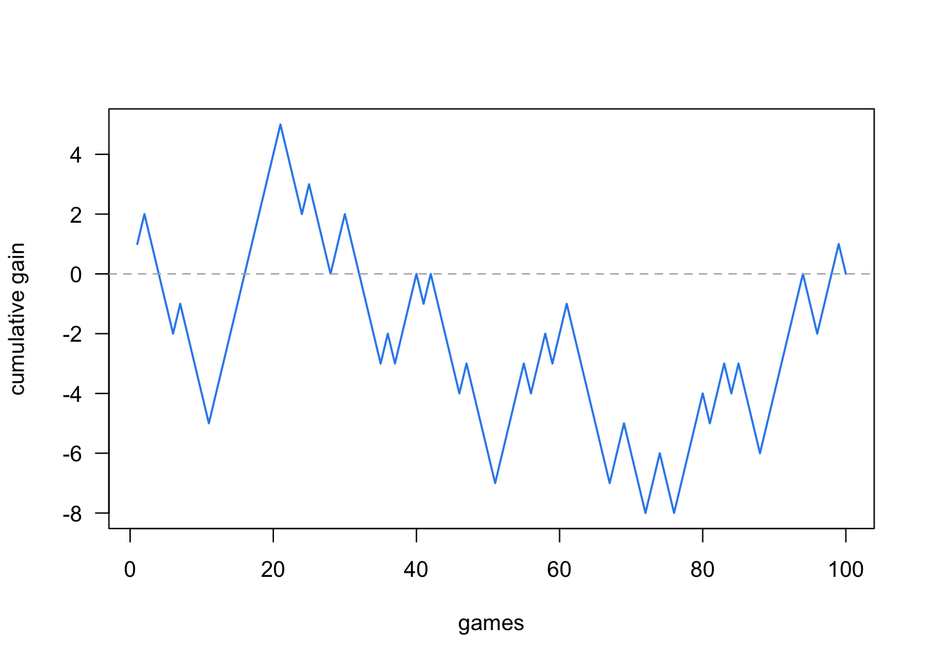

Observe where the blue line ends at game 100: exactly at a y-axis value of zero. Basically, in this series of 100 games, you didn’t gain any money, but you didn’t lose either.

5.2.2 Cumulative Gains with ggplot2

What if you prefer to make a graphic with "ggplot2" functions instead of using the traditional base plot() approach? No problem, this is also possible.

We are assuming that you have loaded the package "tidyverse" which contains "ggplot2".

library(tidyverse)   # which contains ggplot2

To make graphics with ggplot(), we first need to assemble the data to be plotted into a data frame. One way to create this table is as follows:

tbl = data.frame(
  game = 1:number_games,
  gain = gains,
  cumulative_gain = cumsum(gains)
)

head(tbl)

##   game gain cumulative_gain
## 1    1    1               1
## 2    2    1               2
## 3    3   -1               1
## 4    4   -1               0
## 5    5   -1              -1
## 6    6   -1              -2

Having the appropriate data in a data frame object tbl, we can now proceed to make a line graph with the number game in the x-axis, and the cumulative gain in the y-axis.

ggplot(data = tbl, aes(x = game, y = cumulative_gain)) + 
  geom_hline(yintercept = 0, color = "gray70") +
  geom_line(color = "#318BEC", size = 1) +
  labs(x = "games", 
       y = "cumulative gain", 
       title = "Playing Game-A 100 times",
       subtitle = "Sequence of cumulative gains") +
  theme_minimal()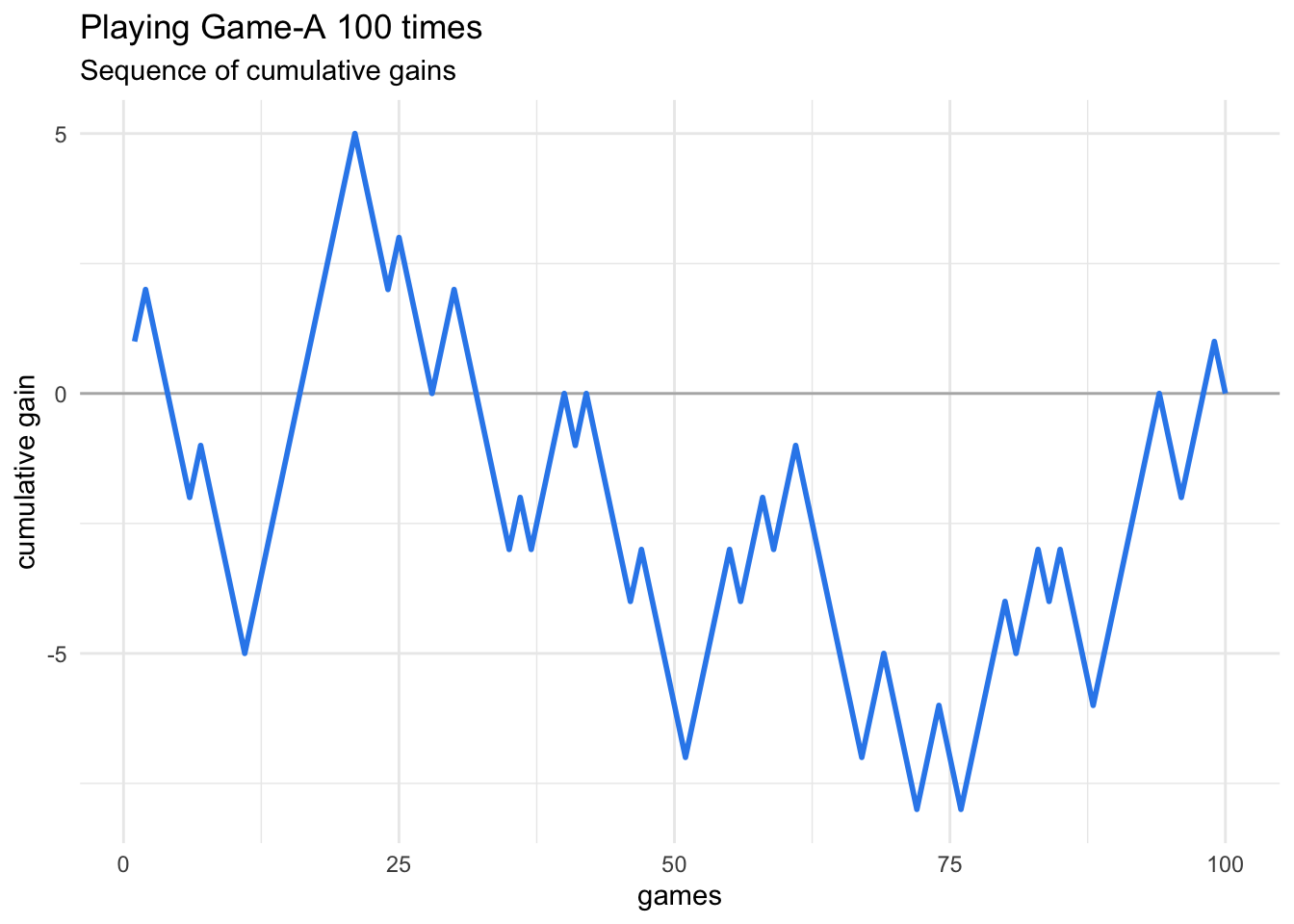

5.2.3 Animated ggplot graphic

For your amusement, it is also possible to make an animated ggplot graphic. This requires the companion package "gganimate"

library(gganimate)

# gganimate may also need:
# library(gifski)   # for gif output
# library(av)       # for video output

For convenience purposes, it’s better if we assign the graphic to an object, e.g. static_plot, and then we add a transition layer with one of the transition_() functions. In this example we are going to use the transition_reveal() function, specifying game as the variable in the data tbl that needs to be taken into account to create the frames of the animation.

# ggplot object
static_plot = ggplot(data = tbl, aes(x = game, y = cumulative_gain)) + 
  geom_hline(yintercept = 0, color = "gray70") +
  geom_line(color = "#318BEC", size = 1) +
  labs(x = "games", 
       y = "cumulative gain", 
       title = "Playing Game-A 100 times",
       subtitle = "Sequence of cumulative gains") +
  theme_minimal()

# animation
animated_plot = static_plot +
  transition_reveal(game)

animate(animated_plot)

To save the animated plot into a gif file, you use anim_save(), for example:

# save gif in working directory
anim_save(
  filename = "Playing-Game-A-100-times.gif", 
  animation = animated_plot,
  height = 5, 
  width = 7, 
  units = "in",
  res = 200)