6 Running Various Simulations

A single series of 100 games may not be enough to fully understand the probability behavior of Game-A. So let’s see how to run various simulations, all of them involving playing 100 games.

Let’s start small. Meaning, let’s begin with a handful of games, and a few simulations. This will allow us to get a better idea of the objects and commands we need to use in order to later generalize things with more games and simulations.

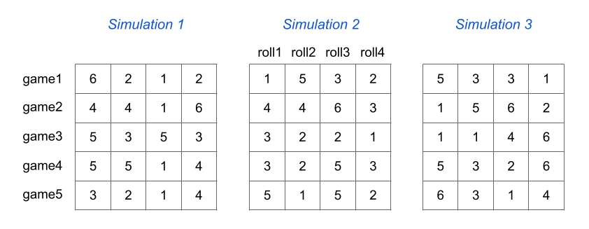
Our starting point will involve 3 simulations, each one consisting of 5 games as illustrated in the picture below.

Here’s some naive code to run these simulations. We are momentarily considering this piece of code to get a high-level intuition of the things we might need later to write more efficient commands.

# -------------------------------------
# three simulations, each of 5 games
# -------------------------------------

set.seed(753)

# main inputs
die = 1:6
number_games = 5

# simulation 1
games_sim1 = matrix(0, nrow = number_games, ncol = 4)
for (game in 1:number_games) {
  games_sim1[game, ] = sample(die, size = 4, replace = TRUE)
}
wins_sim1 = apply(games_sim1, 1, function(x) any(x == 6))
prop_wins_sim1 = sum(wins_sim1) / number_games


# simulation 2
games_sim2 = matrix(0, nrow = number_games, ncol = 4)
for (game in 1:number_games) {
  games_sim2[game, ] = sample(die, size = 4, replace = TRUE)
}
wins_sim2 = apply(games_sim2, 1, function(x) any(x == 6))
prop_wins_sim2 = sum(wins_sim2) / number_games


# simulation 3
games_sim3 = matrix(0, nrow = number_games, ncol = 4)
for (game in 1:number_games) {
  games_sim3[game, ] = sample(die, size = 4, replace = TRUE)
}
wins_sim3 = apply(games_sim3, 1, function(x) any(x == 6))
prop_wins_sim3 = sum(wins_sim3) / number_games


# summary: proportion of wins
c('sim1' = prop_wins_sim1,
  'sim2' = prop_wins_sim2,
  'sim3' = prop_wins_sim3)

## sim1 sim2 sim3 
##  0.4  0.2  0.8

This piece of code has a lot of unnecessary redundancy. But let’s ignore this fact for a second. In each simulation, we create a matrix games_sim to store the rolls of each game. Then we use apply() to determine which games are wins (wins_sim), and finally we calculate the proportion of wins (prop_wins_sim).

If you inspect the vectors wins_sim1, wins_sim2, and wins_sim3, you’ll see that these are of "logical" data-type. TRUE means that a given game is a win, whereas FALSE means lose.

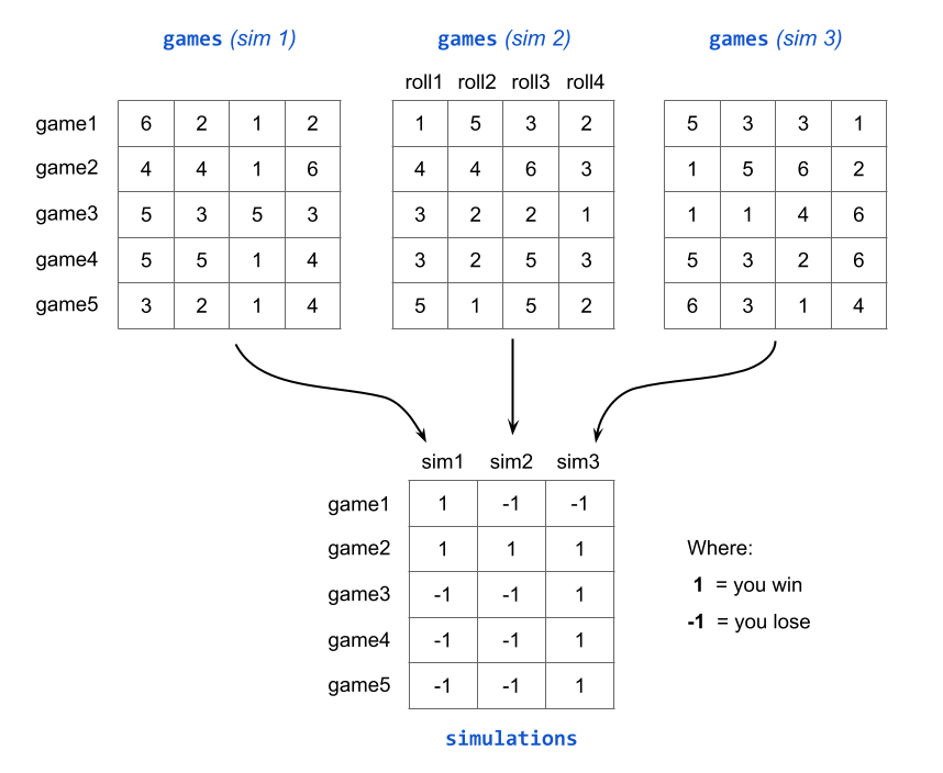
Alternatively, instead of dealing with the logical vectors wins_sim, we can convert their values into numbers: 1 instead of TRUE, and -1 instead of FALSE. Why do we need this change from logical to numbers? Quick answer, you don’t really need it. But as we’ll see, working with 1 and -1 is more convenient later down the road when we calculate cumulative gains.

The diagram below depicts this idea of storing the end result of each game into 1 (win) or -1 (lose), for every simulation:

6.1 Embedded `for()` loops

Let’s take the preceding naive code and try to make it more compact. We are going to use embedded for() loops: one of them to take care of the simulations, and the other one to take care of the games.

The idea is to iterate through each simulation: 1, 2, and 3. And then, in a given simulation, we iterate through each game: 1, 2, 3, 4, and 5.

set.seed(753)

# main inputs
die = 1:6
number_games = 5
number_sims = 3

# matrix to store simulation outputs
simulations = matrix(0, nrow = number_games, ncol = number_sims)

# 1st loop) iterate through each simulation
for (sim in 1:number_sims) {
  games = matrix(0, nrow = number_games, ncol = 4)
  
  # 2nd loop) iterate through each game
  for (game in 1:number_games) {
    games[game, ] = sample(die, size = 4, replace = TRUE)
  }
  any_sixes = apply(games, 1, function(x) any(x == 6))
  simulations[ ,sim] = ifelse(any_sixes, 1, -1)
}

rownames(simulations) = paste0("game", 1:number_games)
colnames(simulations) = paste0("sim", 1:number_sims)
simulations

##       sim1 sim2 sim3
## game1    1   -1   -1
## game2    1    1    1
## game3   -1   -1    1
## game4   -1   -1    1
## game5   -1   -1    1

What’s going on with this code? Before starting the iterations, we create a matrix simulations which will store the numeric values of all games, and all simulations. The rows of this matrix are associated to the games, and the columns are associated to the simulations. At the end of the iterative process, the cells of this matrix will be populated with either 1 (win game) and -1 (lose game).

The first for() loop—the outer loop—iterates through the simulations. At the beginning of each simulation, an auxiliary games matrix is initialized, which then gets populated in the embedded for() loop. This second for() loop—the inner loop—iterates through the games, obtaining the rolls of the five games. Right after the games are completed in the inner loop, we use apply() to determine which games are wins (i.e. have at least one 6), and then we convert the TRUE’s and FALSE’s into 1 and -1, respectively, by using ifelse(). This numeric vector is stored in the corresponding column of the simulations matrix.

Having obtained the matrix simulations, we then proceed to count the number of wins total_wins (see code below). Notice the use of apply() to count the number of wins for each column of simulations. The last step involves computing the proportion of wins prop_wins:

total_wins = apply(simulations, 2, function(x) sum(x==1))
prop_wins = total_wins / number_games
prop_wins

## sim1 sim2 sim3 
##  0.4  0.2  0.8

6 Running Various Simulations

6.1 Embedded for() loops

6.1 Embedded `for()` loops