1 Let’s Toss a Coin
To illustrate the concepts behind object-oriented programming in R, we are going to consider a classic chance process (or chance experiment) of flipping a coin.
In this chapter you will learn how to implement code in R that simulates tossing a coin one or more times.
1.1 Coin object
Think about a standard coin with two sides: heads and tails.

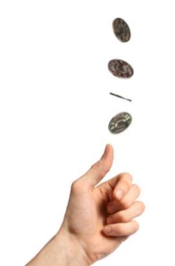
Figure 1.1: two sides of a coin
To toss a coin using R, we first need an object that plays the role of a coin.
How do you create such a coin? Perhaps the simplest way to create a coin with
two sides, "heads" and "tails", is with a character vector via the combine
function c():
You can also create a numeric coin that shows 1 and 0 instead of
"heads" and "tails":
Likewise, you can also create a logical coin that shows TRUE and FALSE
instead of "heads" and "tails":
1.2 Tossing a coin
Once you have an R object that represents a coin, the next step involves learning how to simulate tossing the coin.
The important thing to keep in mind is that tossing a coin is a random
experiment: you either get heads or tails. One way to simulate the action of
tossing a coin in R is with the function sample() which lets you draw random
samples, with or without replacement, of the elements in the input vector.
Here’s how to simulate a coin toss using sample() to take a random sample of
size 1 of the elements in coin:
You use the argument size = 1 to specify that you want to take a sample of
size 1 from the input vector coin.
1.2.1 Random Samples
By default, sample() takes a sample of the specified size
without replacement. If size = 1, it does not really matter whether the
sample is done with or without replacement.
To draw two elements without replacement, use sample() like this:
This is equivalent to calling sample() with the argument replace = FALSE:
What if you try to toss the coin three or four times?
Notice that R produced an error message:
Error in sample.int(length(x), size, replace, prob): cannot take a
sample larger than the population when 'replace = FALSE'
This is because the default behavior of sample() cannot draw more elements
than the length of the input vector.
To be able to draw more elements, you need to sample with replacement, which
is done by specifying the argument replace = TRUE, like this:
1.3 The Random Seed
The way sample() works is by taking a random sample from the input vector.
This means that every time you invoke sample() you will likely get a different
output. For instance, when we run the following command twice, the output of
the first call is different from the output in the second call, even though the
command is exactly the same in both cases:
# another five tosses
sample(coin, size = 5, replace = TRUE)
#> [1] "heads" "heads" "heads" "heads" "tails"
In order to make the examples replicable (so you can get the same output as mine),
you need to specify what is called a random seed. This is done with the
function set.seed(). By setting a seed, every time you use one of the random
generator functions, like sample(), you will get the same values.
1.4 Sampling with different probabilities
Last but not least, sample() comes with the argument prob which allows you
to provide specific probabilities for each element in the input vector.
By default, prob = NULL, which means that every element has the same probability
of being drawn. In the example of tossing a coin, the command sample(coin) is
equivalent to sample(coin, prob = c(0.5, 0.5)). In the latter case we
explicitly specify a probability of 50% chance of heads, and 50% chance of tails:
# tossing a fair coin
coin <- c("heads", "tails")

sample(coin)
#> [1] "tails" "heads"

# equivalent
sample(coin, prob = c(0.5, 0.5))
#> [1] "tails" "heads"
However, you can provide different probabilities for each of the elements in the
input vector. For instance, to simulate a loaded coin with chance of heads
20%, and chance of tails 80%, set prob = c(0.2, 0.8) like so:
# tossing a loaded coin (20% heads, 80% tails)
sample(coin, size = 5, replace = TRUE, prob = c(0.2, 0.8))
#> [1] "heads" "tails" "tails" "tails" "tails"
1.4.1 Simulating tossing a coin
Now that we have all the elements to toss a coin with R, let’s simulate flipping
a coin 100 times, and then use the function table() to count the resulting
number of "heads" and "tails":
# number of flips
num_flips <- 100

# flips simulation
coin <- c('heads', 'tails')
flips <- sample(coin, size = num_flips, replace = TRUE)

# number of heads and tails
freqs <- table(flips)
freqs
#> flips
#> heads tails
#>    50    50
In my case, I got 50 heads and 50 tails. Your results will
probably be different than mine. Sometimes you will get more "heads", sometimes
you will get more "tails", and sometimes you will get exactly 50 "heads"
and 50 "tails".
Let’s run another series of 100 flips, and find the frequency of "heads" and
"tails" with the help of the table() function:
# one more 100 flips
flips <- sample(coin, size = num_flips, replace = TRUE)
freqs <- table(flips)
freqs
#> flips
#> heads tails
#>    50    50
To make things more interesting, let’s consider how the frequency of heads
evolves over a series of n tosses (in this case n = num_flips).
With the vector heads_freq, we can graph the (cumulative) relative frequencies
with a line-plot:
plot(heads_freq,      # vector
     type = 'l',      # line type
     lwd = 2,         # width of line
     col = 'tomato',  # color of line
     las = 1,         # orientation of tick-mark labels
     ylim = c(0, 1),  # range of y-axis
     xlab = "number of tosses",    # x-axis label
     ylab = "relative frequency")  # y-axis label
abline(h = 0.5, col = 'gray50')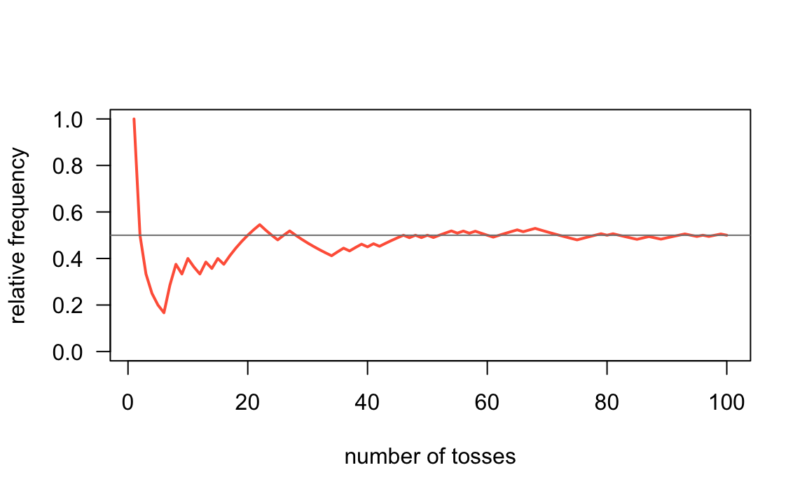
Figure 1.2: Cumulative relative frequencies of heads