10 Matrices and Arrays
In the previous four chapters, we discussed a number of ideas and concepts that basically have to do with vectors and their cousins factors. You can think of vectors and factors as one-dimensional objects. While many data sets can be handled through vectors and factors, there are occasions in which one dimension is not enough. The classic example for when one-dimensional objects are not enough involves working with data that fits better into a tabular structure consisting of a series of rows (one dimension) and columns (another dimension).
In this chapter we introduce R arrays, which are multidimensional atomic
objects including 2-dimensional arrays better known as matrices, and
N-dimensional generic arrays.
10.1 Motivation
Let us continue discussing the savings-investing scenario in which you deposit $1000 into a savings account that pays you an annual interest rate of 2%.
Assuming that you leave that money in the bank for several years, with a constant rate of return \(r\), you can use the Future Value (FV) formula to calculate how much money you’ll have at the end of year \(n\):
\[ \text{FV} = \text{PV} (1 + r)^n \]
where:
- \(\text{FV}\) = future value
- \(\text{PV}\) = present value
- \(\text{r}\) = annual interest rate
- \(\text{n}\) = number of years
Here’s some R code to obtain a vector amounts containing the amount of money
that you would have from the beginning of time, and at the end of every year
during a 5 year period:
# inputs
deposit = 1000
rate = 0.02
years = 0:5

# future values
amounts = deposit * (1 + rate)^years
amounts
> [1] 1000.000 1020.000 1040.400 1061.208 1082.432
> [6] 1104.081
Recall that this code is an example of vectorized (and recycling) code because the FV formula is applied to all the elements of the involved vectors, some of which have different lengths.
So far, so good.
Now, consider a seemingly simple modification. What if you want to organize the amount values in a table? Something like this:
| year | amount |
|---|---|
| 0 | 1000.000 |
| 1 | 1020.000 |
| 2 | 1040.400 |
| 3 | 1061.208 |
| 4 | 1082.432 |
| 5 | 1104.081 |
In other words, what if you are interested not in getting the set of future
values in a vector, but instead you want them to be arranged in some sort of
tabular object? How can you create a table in which the first column year
corresponds to the years, and the second column amount corresponds to the
future amounts? Let’s find out.
10.2 Matrices
R provides two main ways to organize data in a tabular (i.e. rectangular)
object. One of them is a matrix—the topic of this chapter—and the other
one is a data.frame—to be discussed in a subsequent chapter.
Creating a matrix by column-binding vectors
You can build a matrix by column binding vectors using the function
cbind(). In the code below we pass years and amount to the cbind()
function, which returns a matrix having the tabular structure that we are
looking for: years in the first column, and amounts in the second column.
# inputs
deposit = 1000
rate = 0.02
years = 0:5

# future values
amounts = deposit * (1 + rate)^years

# output as a matrix via cbind()
savings = cbind(years, amounts)
savings
>      years  amounts
> [1,]     0 1000.000
> [2,]     1 1020.000
> [3,]     2 1040.400
> [4,]     3 1061.208
> [5,]     4 1082.432
> [6,]     5 1104.081
As you can tell, the use of cbind() is straightforward. All you have to do
is pass the vectors, separating them with a comma. Each vector will become a
column of the returned matrix.
Creating a matrix by row-binding vectors
You can also build a matrix by row binding vectors. For instance, pretend
for a minute that we are interested in obtaining a tabular object in which
the first row corresponds to years, and the second row to amounts. To
obtain this object we use rbind() as follows:
savings = rbind(years, amounts)
savings
>         [,1] [,2]   [,3]     [,4]     [,5]
> years      0    1    2.0    3.000    4.000
> amounts 1000 1020 1040.4 1061.208 1082.432
>             [,6]
> years      5.000
> amounts 1104.081
The difference between cbind() and rbind() is that the latter will “stack”
the given vectors on top of each other. That is, each vector will become a row
of the returned matrix.
10.2.1 What kind of object is a matrix?
In turns out that an R matrix is a special type of multi-dimensional atomic
object called array. Both classes of objects, together with vectors and
factors, form the triad of atomic objects. This is illustrated in the following
diagram in terms of their number of dimensions.
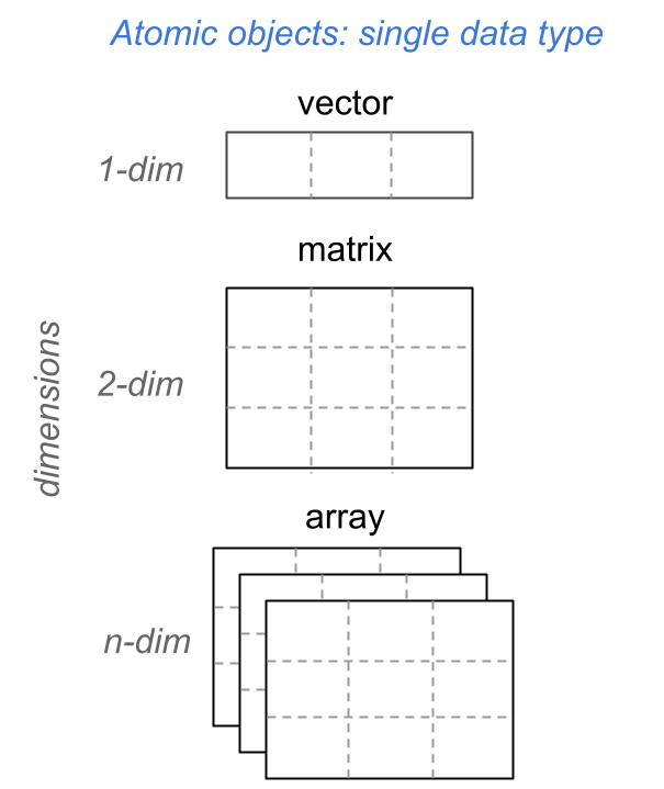
Figure 10.1: Triad of atomic data objects in R.
Personally, I prefer to reserve the term array for three or more dimensional
arrays. As you can tell from the above diagram, this is how I’m using this
term in the book. However, you should always keep in mind that a matrix is an
array. The other way around is not necessarily true: not all arrays are
matrices.
10.3 Creating matrices with matrix()
The cbind() and rbind() functions provide a convenient way to create
matrices from different input vectors. But the kind of matrices that you can
create with them is limited if all you have is just one input vector.
So, in addition to cbind() and rbind(), R comes with the function matrix()
which is the workhorse function for creating matrices. Usually, you provide
an input vector, and also the number of rows and columns (i.e. the
matrix dimensions) that the returned matrix should have.
Here is how to use matrix() to create the savings matrix that we are
interested in obtaining:
savings = matrix(c(years, amounts), nrow = 6, ncol = 2)
savings
>      [,1]     [,2]
> [1,]    0 1000.000
> [2,]    1 1020.000
> [3,]    2 1040.400
> [4,]    3 1061.208
> [5,]    4 1082.432
> [6,]    5 1104.081
This is an interesting piece of code. Notice that years and amounts are
combined into a single vector, which is the main input of matrix(). The two
other arguments correspond to the matrix dimensions: nrow = 6 tells R that
we want to produce a matrix with 6 rows; ncol = 2 indicates that we want the
matrix to have 2 columns.
10.3.1 Column-Major Matrices
When creating a matrix via the function matrix(), R takes into consideration
three important aspects:
the length of the input vector.
the “size” of the matrix given by its number of rows and columns; think of this as the total number of cells or entries in the matrix.
whether the length of the input vector is a multiple or sub-multiple of the size of the matrix.
In the current example, the input vector c(years, amounts) has 12 elements.
In turn, the size of the desired matrix is given by the multiplication of the
number of rows (2) times the number of columns (6), that is:
\[ \text{size of matrix} = 6 \times 2 = 12 \text{ cells} \]
R then compares the length of the input vector against the size of the matrix. If these numbers are the same, like in this example, R proceeds to split the elements of the input vector into 2 sections or sub-vectors, each one containing 6 elements. Each of these sections will become a column of the output matrix.
In other words, the vector c(years, amounts) is split into 2 sub-vectors:
# the first sub-vector is:
0  1  2  3  4  5

# the second sub-vector is:
1000.000  1020.000  1040.400  1061.208  1082.432  1104.081
The first sub-vector, which corresponds to years, becomes the first column.
The second sub-vector, which corresponds to amounts, becomes the second
column. In technical terms we say that R matrices are stored
column-major because of the mechanism used by R to arrange the elements of
an input vector in order to create a matrix.
Mismatch between length of input vector and size of matrix
What about those cases in which the length of the input vector does not match the size of the desired matrix? For example, consider the following commands illustrating this type of situation:
# examples in which length of input vector
# does not match size of matrix
m1 = matrix(1:3, nrow = 3, ncol = 2)

m2 = matrix(1:3, nrow = 2, ncol = 3)

m3 = matrix(1:12, nrow = 3, ncol = 2)
> Warning in matrix(1:12, nrow = 3, ncol = 2): data
> length differs from size of matrix: [12 != 3 x 2]

m4 = matrix(1:4, nrow = 3, ncol = 2)
> Warning in matrix(1:4, nrow = 3, ncol = 2): data
> length [4] is not a sub-multiple or multiple of
> the number of rows [3]

m5 = matrix(1:8, nrow = 2, ncol = 3)
> Warning in matrix(1:8, nrow = 2, ncol = 3): data
> length [8] is not a sub-multiple or multiple of
> the number of columns [3]
In matrices m1 and m2 the input vector 1:3 is a sub-multiple of the size
of the matrix 6.
In matrix m3 the input vector 1:12 is longer than the size of the matrix: 6.
However, the entire length of the vector, 12, is a multiple of the size 6.
In matrices m4 and m5, all the input vectors have lengths that are
neither a multiple or sub-multiple of the size of the returned matrix.
When the length of the input vector does not match the size of the desired
matrix, R applies its recycling rules. Let’s pay attention to m1:
m1
>      [,1] [,2]
> [1,]    1    1
> [2,]    2    2
> [3,]    3    3
Note how the values of the input vector 1:3 are recycled to form the columns
of m1. The values appear in the first column, but they also appear in the
second column after being recycled.
In contrast, matrix m3 does not use all the elements in the input vector
1:12. Instead, only the first six values are retained.
As for the matrices m4 and m5, they all have an input vector whose
length is neither a multiple nor a sub-multiple of the size of the matrix.
In these cases R will also apply its recycling rules, but it will also display
a warning message letting us know that the length of the input vector is not a
multiple or sub-multiple of either the number of rows or the number of columns.
10.3.2 Giving names to rows and columns
Often, you may need to provide names for either the rows and/or the columns of
a matrix. R comes with the functions rownames() and colnames() that can be
used to assign names for the rows and columns, for example:
# matrix of savings amounts
savings = matrix(c(years, amounts), nrow = 6, ncol = 2)

# row and columns names
rownames(savings) = 1:6
colnames(savings) = c("year", "amount")

savings
>   year   amount
> 1    0 1000.000
> 2    1 1020.000
> 3    2 1040.400
> 4    3 1061.208
> 5    4 1082.432
> 6    5 1104.081
10.3.3 More Matrices
Let’s make things a bit more complex. Say you have the following investments:
$1000 in a savings account that pays 2% annual return, during 4 years
$2000 in a money market account that pays 2.5% annual return, during 2 years
$5000 in a certificate of deposit that pays 3% annual return, during 3 years
In R, we can calculate the future values of each type of investment product:
# savings account
savings = 1000 * (1 + 0.02)^(0:4)
savings
> [1] 1000.000 1020.000 1040.400 1061.208 1082.432
# money market
moneymkt = 2000 * (1 + 0.025)^(0:2)
moneymkt
> [1] 2000.00 2050.00 2101.25# certificate of deposit
certificate = 5000 * (1 + 0.03)^(0:3)
certificate
> [1] 5000.000 5150.000 5304.500 5463.635Separated matrices
We can create individual matrices for each type of account:
# savings account
sav_mat = cbind(0:4, savings)
# money market
mm_mat = cbind(0:2, moneymkt)# certificate of deposit
cd_mat = cbind(0:3, certificate)Single matrix
Alternatively, we can stack everything into a single matrix:
cbind(c(0:4, 0:2, 0:3), c(savings, moneymkt, certificate))
>       [,1]     [,2]
>  [1,]    0 1000.000
>  [2,]    1 1020.000
>  [3,]    2 1040.400
>  [4,]    3 1061.208
>  [5,]    4 1082.432
>  [6,]    0 2000.000
>  [7,]    1 2050.000
>  [8,]    2 2101.250
>  [9,]    0 5000.000
> [10,]    1 5150.000
> [11,]    2 5304.500
> [12,]    3 5463.635
What about mixing data types?
What if you want some table like this:
| account | year | amount |
|---|---|---|
| savings | 0 | 1000.000 |
| savings | 1 | 1020.000 |
| savings | 2 | 1040.400 |
| savings | 3 | 1061.208 |
| savings | 4 | 1082.432 |
| moneymkt | 0 | 2000.000 |
| moneymkt | 1 | 2050.000 |
| moneymkt | 2 | 2101.250 |
| certif | 0 | 5000.000 |
| certif | 1 | 5150.250 |
| certif | 2 | 5304.500 |
| certif | 3 | 5463.635 |
We could use the cbind() function in an attempt to obtain a matrix having
a similar rectangular structure as in the above table:
investments = cbind(
  rep(c("savings", "moneymkt", "certif"), times = c(5, 3, 4)),
  c(0:4, 0:2, 0:3),
  c(savings, moneymkt, certificate))

investments
>       [,1]       [,2] [,3]
>  [1,] "savings"  "0"  "1000"
>  [2,] "savings"  "1"  "1020"
>  [3,] "savings"  "2"  "1040.4"
>  [4,] "savings"  "3"  "1061.208"
>  [5,] "savings"  "4"  "1082.43216"
>  [6,] "moneymkt" "0"  "2000"
>  [7,] "moneymkt" "1"  "2050"
>  [8,] "moneymkt" "2"  "2101.25"
>  [9,] "certif"   "0"  "5000"
> [10,] "certif"   "1"  "5150"
> [11,] "certif"   "2"  "5304.5"
> [12,] "certif"   "3"  "5463.635"
Do you notice something funny with the matrix investments?
As you can tell, all the values in investments are displayed being surrounded
with double quotes. This indicates that all the values are of type character.
Why is this?
Recall that matrices are atomic objects. Usually, you provide an input vector containing the elements to be arranged into a rectangular array with a certain number of rows and columns. Because vectors are atomic, this property is “inherited” by the returned matrix.
It turns out that you can use other classes of data objects, not necessarily atomic, for creating a matrix. If the input object is non-atomic, R will coerce it into a vector, making the input an atomic object.
So either way, whether you provide an atomic input or a non-atomic input,
to any of the matrix-creation functions, R will always produce an atomic
output. This is the reason why the below command produces a character matrix:
investments = cbind(
  rep(c("savings", "moneymkt", "certif"), times = c(5, 3, 4)),
  c(0:4, 0:2, 0:3),
  c(savings, moneymkt, certificate))

typeof(investments)
> [1] "character"
The three input vectors are coerced into a single vector of character data
type, causing the investments matrix to be of type character.