7+ ways to plot dendrograms in R

Posted on October 03, 2012

Today we are going to talk about the wide spectrum of functions and methods that we can use to visualize dendrograms in R. You can check an extended version of this post with the complete reproducible code in R in this Rpub.

A quick reminder: a dendrogram (from Greek dendron=tree, and gramma=drawing) is nothing more than a tree diagram that practitioners use to depict the arrangement of the clusters produced by hierarchical clustering.

1) Basic dendrograms

Let’s start with the most basic type of dendrogram. For that purpose we’ll use the mtcars dataset and we’ll calculate a hierarchical clustering with the function hclust() (with the default options).

# prepare hierarchical cluster
hc = hclust(dist(mtcars))

# very simple dendrogram
plot(hc)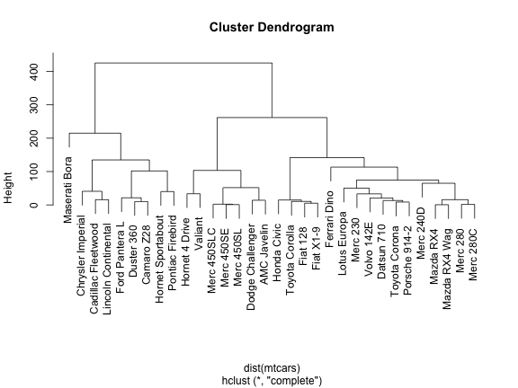

# labels at the same level
plot(hc, hang = -1)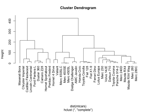

2) A less basic dendrogram

In order to add more format to the dendrograms like the one above, we simply need to tweek the right parameters.

# set background color
op = par(bg = "#DDE3CA")
# plot dendrogram
plot(hc, col = "#487AA1", col.main = "#45ADA8", col.lab = "#7C8071",
     col.axis = "#F38630", lwd = 3, lty = 3, sub = '', hang = -1, axes = FALSE)
# add axis
axis(side = 2, at = seq(0, 400, 100), col = "#F38630",
     labels = FALSE, lwd = 2)
# add text in margin
mtext(seq(0, 400, 100), side = 2, at = seq(0, 400, 100),
      line = 1, col = "#A38630", las = 2)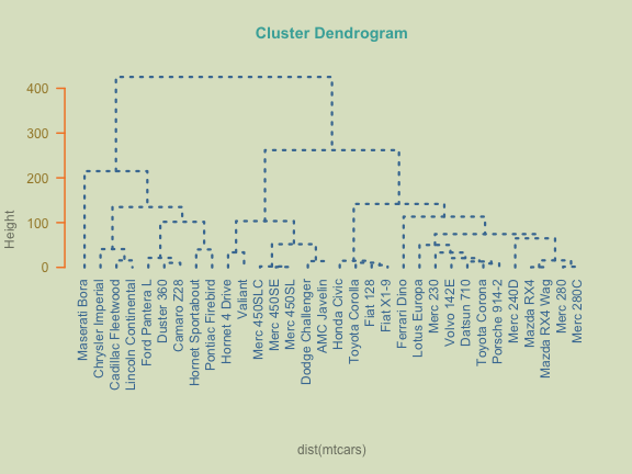

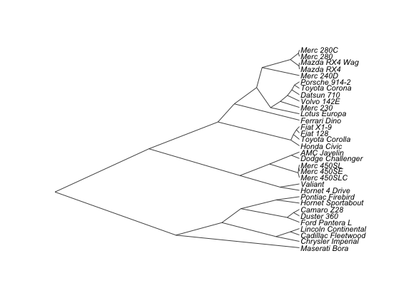
par(op)

An alternative way to produce dendrograms is to specifically convert "hclust" objects into "dendrograms" objects.

# using dendrogram objects
hcd = as.dendrogram(hc)

# alternative way to get a dendrogram
op = par(mfrow = c(2, 1))
plot(hcd)

# triangular dendrogram
plot(hcd, type = "triangle")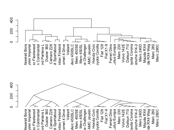

par(op)

3) Zooming-in on dendrograms

Another very useful option is the ability to inspect selected parts of a given tree. For instance, if we wanted to examine the top partitions of the dendrogram, we could cut it at a height of 75

# plot dendrogram with some cuts
op = par(mfrow = c(2, 1))
plot(cut(hcd, h = 75)$upper, main = "Upper tree of cut at h=75")

plot(cut(hcd, h = 75)$lower[[2]],
     main = "Second branch of lower tree with cut at h=75")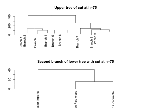

par(op)

4) More customizable dendrograms

In order to get more customized graphics we need a little bit of more code. A very useful resource is the function dendrapply() that can be used to apply a function to all nodes of a dendrgoram. This comes very handy if we want to add some color to the labels.

# vector of colors
labelColors = c("#CDB380", "#036564", "#EB6841", "#EDC951")

# cut dendrogram in 4 clusters
clusMember = cutree(hc, 4)

# function to get color labels
colLab <- function(n) {
  if (is.leaf(n)) {
    a <- attributes(n)
    labCol <- labelColors[clusMember[which(names(clusMember) == a$label)]]
    attr(n, "nodePar") <- c(a$nodePar, lab.col = labCol)
  }
  n
}

# using dendrapply
clusDendro = dendrapply(hcd, colLab)

# make plot
plot(clusDendro, main = "Cool Dendrogram", type = "triangle")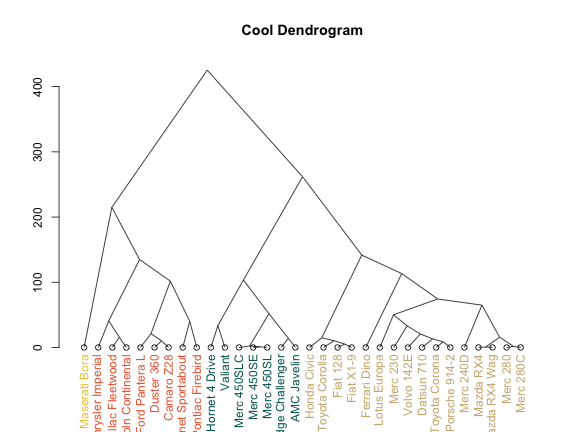

5) Phylogenetic trees

Closely related to dendrograms, phylogenetic trees are another option to display tree diagrams showing the relationships among observations based upon their similarities.

A very nice tool for displaying more appealing trees is provided by the R package "ape". In this case, what we need is to convert the "hclust" objects into "phylo" objects with the funtions as.phylo(). The plot.phylo() function has four more different types for plotting a dendrogram. Here they are:

# load package ape;
# remember to install it: install.packages("ape")
library(ape)
# plot basic tree
plot(as.phylo(hc), cex = 0.9, label.offset = 1)
# cladogram
plot(as.phylo(hc), type="cladogram", cex = 0.9, label.offset = 1)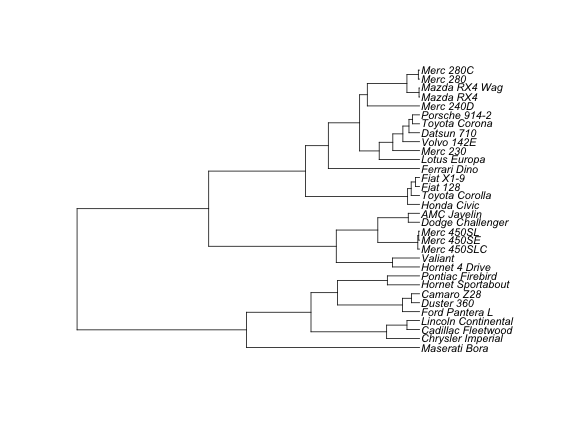

# unrooted
plot(as.phylo(hc), type = "unrooted")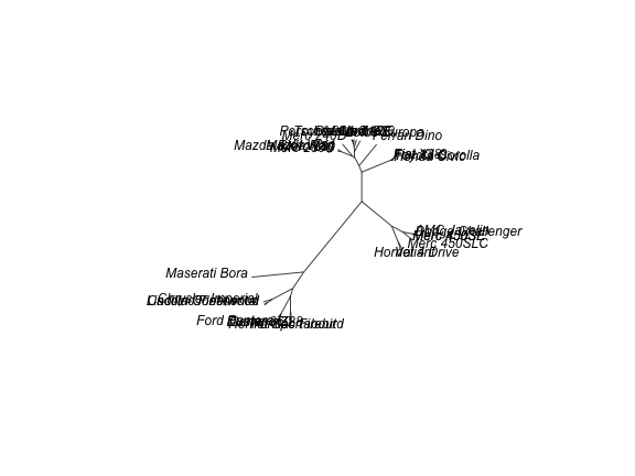

# fan
plot(as.phylo(hc), type = "fan")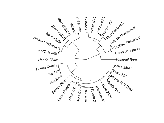

# radial
plot(as.phylo(hc), type = "radial")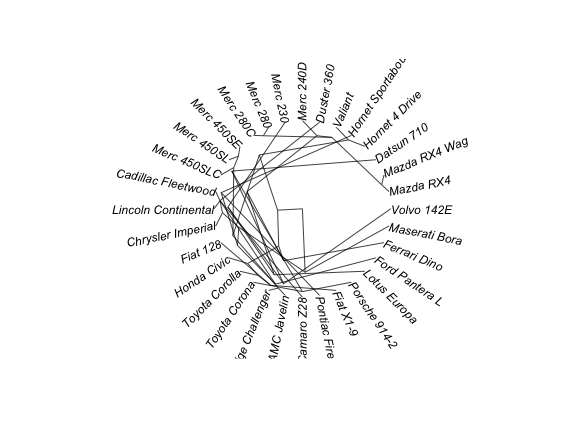

What I really like about the ape package is that we have more control on the appearance of the dendrograms, being able to customize them in different ways. For example, we can tweek some parameters according to our needs

# vector of colors
mypal = c("#556270", "#4ECDC4", "#1B676B", "#FF6B6B", "#C44D58")
# cutting dendrogram in 5 clusters
clus5 = cutree(hc, 5)
# plot
op = par(bg="#E8DDCB")
# Size reflects miles per gallon
plot(as.phylo(hc), type = "fan", tip.color = mypal[clus5], label.offset = 1,
cex = log(mtcars$mpg,10), col = "red")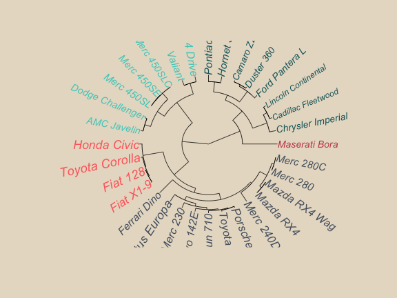

par(op)

6) Dendrograms with ggdendro

For reasons that are unknown to me, the The R package "ggplot2" have no functions to plot dendrograms. However, the ad-hoc package "ggdendro" offers a decent solution. You would expect to have more customization options, but so far they are rather limited. Anyway, for those of us who are ggploters this is another tool in our toolkit.

# remember to install the package: install.packages("ggdendro")
library(ggplot2)
library(ggdendro)

# basic option
ggdendrogram(hc, theme_dendro = FALSE)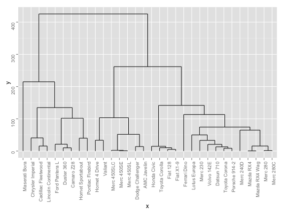

# another option
ggdendrogram(hc, rotate = TRUE, size = 4, theme_dendro = FALSE)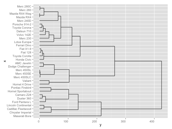

7) Colored dendrogram

Last but not least, there’s one more resource available from Romain Francois’s addicted to R gallery which I find really interesting. The code in R for generating colored dendrograms, which you can download and modify if wanted so, is available here

# load code of A2R function
source("http://addictedtor.free.fr/packages/A2R/lastVersion/R/code.R")

# colored dendrogram
op = par(bg = "#EFEFEF")
A2Rplot(hc, k = 3, boxes = FALSE, col.up = "gray50",
        col.down = c("#FF6B6B", "#4ECDC4", "#556270"))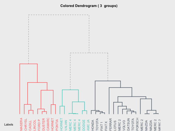

par(op)

For a more detailed version of the code presented in this post, check this Rpub.