7 Functions to do Metric Multidimensional Scaling in R

Posted on January 23, 2013

In this post we will talk about 7 different ways to perform a metric multidimensional scaling in R.

Multidimensional Scaling

Multidimensional Scaling (MDS), is a set of multivariate data analysis methods that are used to analyze similarities or dissimilarities in data. One of the nice features of MDS is that it allows us to represent the (dis)similarities among pairs of objects as distances between points in a low-dimensional space. Put another way, MDS allows us to visualize the (dis)similarities in a low-dimensional space for exploration and inspection purposes.

The general approach behind MDS consists of calculating a (dis)similarity matrix among pairs of objects (i.e. observations, individuals, samples, etc), and then apply one of the several MDS “models” to obtain the low-dimensional representation. The MDS model to be applied depends on the type of data, and consequently, the type of (dis)similarity measurement that the analyst decides to use.

Metric Multidimensional Scaling

Depending on the chosen measurement and the obtained (dis)similarity matrix, MDS can be divided in two main approaches: metric and nonmetric. If the analyzed matrix is based on a metric distance, we talk about metric MDS, otherwise we talk about nonmetric MDS.

Metric multidimensional scaling, also known as Principal Coordinate Analysis or Classical Scaling, transforms a distance matrix into a set of coordinates such that the (Euclidean) distances derived from these coordinates approximate as well as possible the original distances (do not confuse Principal Coordinate Analysis with Principal Component Analysis). In other words, the advantage of working with metric MDS, is that the relationships among objects can, in most cases, be fully represented in an Euclidean space.

Metric Multidimensional Scaling in R

R has a number of ways to perform metric MDS. The following list shows you 7 different functions to perform metric MDS (with their corresponding packages in parentheses):

• cmdscale() (stats by R Development Core Team)
• smacofSym() (smacof by Jan de Leeuw and Patrick Mair)
• wcmdscale() (vegan by Jari Oksanen et al)
• pco() (ecodist by Sarah Goslee and Dean Urban)
• pco() (labdsv by David W. Roberts)
• pcoa() (ape by Emmanuel Paradis et al)
• dudi.pco() (ade4 by Daniel Chessel et al)

You should know that all the previous functions require a distance matrix as the main argument to work with. If you don’t have your data in (dis)similarity matrix format, you can calculate the distance matrix with the function dist(). This is the “work-horse” function in R for calculating distances (e.g. euclidean, manhattan, binary, canberra and maximum). In addition, some of the packages mentioned above provide their own functions for calculating other types of distances.

Installing packages

Except for cmdscale(), the rest of the functions don’t come with the default distribution of R; this means that you have to install their corresponding packages:

# install packages
install.packages(c("vegan", "ecodist", "labdsv", "ape", "ade4", "smacof"))

Once you have installed the packages, you just need to load them:

# load packages
library(vegan)
library(ecodist)
library(labdsv)
library(ape)
library(ade4)
library(smacof)

Data eurodist

We will use the dataset eurodist that gives the road distances (in km) between 21 cities in Europe. Notice that eurodist is already an object of class "dist" (matrix distance). You can inspect the first 5 elements like so:

# convert eurodist to matrix
euromat = as.matrix(eurodist)

# inspect first five elements
euromat[1:5, 1:5]

##           Athens Barcelona Brussels Calais Cherbourg
## Athens         0      3313     2963   3175      3339
## Barcelona   3313         0     1318   1326      1294
## Brussels    2963      1318        0    204       583
## Calais      3175      1326      204      0       460
## Cherbourg   3339      1294      583    460         0

The goal is to apply metric MDS to get a visual representation of the distances between European cities.

1) MDS with cmdscale()

The most popular function to perform a classical scaling is cmdscale() (which comes with the default distribution of R). Its general usage has the following form:

cmdscale(d, k = 2, eig = FALSE, add = FALSE, x.ret = FALSE)

# 1) MDS 'cmdscale'
mds1 = cmdscale(eurodist, k = 2)

# plot
plot(mds1[,1], mds1[,2], type = "n", xlab = "", ylab = "", axes = FALSE,
     main = "cmdscale (stats)")
text(mds1[,1], mds1[,2], labels(eurodist), cex = 0.9, xpd = TRUE)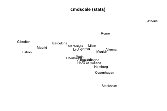

Figure 1: Caption

As you can see, the obtained graphic allows us to represent the distances between cities in a two-dimensional space. However, the representation is not identical to a geographical map of Europe: Athens is in the north while Stockholm is in the south. This “anomaly” reflects the fact that the representation is not unique; if we wanted to get a more accurate geographical representation, we would need to invert the vertical axis.

2) MDS with wcmdscale()

The package "vegan" provides the function wcmdscale() (Weighted Classical Multidimensional Scaling). Its general usage has the following form:

wcmdscale(d, k, eig = FALSE, add = FALSE, x.ret = FALSE, w)

If we specify the vector of the weights w as a vector of ones, wcmdscale() will give ordinary multidimensional scaling.

# 2) MDS 'wcmdscale'
mds2 = wcmdscale(eurodist, k=2, w=rep(1,21))

# plot
plot(mds2[,1], mds2[,2], type = "n", xlab = "", ylab = "",
     axes = FALSE, main = "wcmdscale (vegan)")
text(mds2[,1], mds2[,2], labels(eurodist), cex = 0.9, xpd = TRUE)

3) MDS with pco() (package ecodist)

The package "ecodist" provides the function pco() (Principal Coordinates Analysis). Its general usage has the following form:

pco(x, negvals = "zero", dround = 0)

# 3) MDS 'pco'
mds3 = pco(eurodist)

# plot
plot(mds3$vectors[,1], mds3$vectors[,2], type = "n", xlab = "", ylab = "",
     axes = FALSE, main = "pco (ecodist)")
text(mds3$vectors[,1], mds3$vectors[,2], labels(eurodist), 
     cex = 0.9, xpd = TRUE)

4) MDS with pco() (package labdsv)

The package "labdsv" also provides a function pco() (Principal Coordinates Analysis). Its general usage has the following form:

pco(dis, k = 2)

# 4) MDS 'pco'
mds4 = pco(eurodist, k = 2)

# plot
plot(mds4$points[,1], mds4$points[,2], type = "n", xlab = "", ylab = "",
     axes = FALSE, main = "pco (labdsv)")
text(mds4$points[,1], mds4$points[,2], labels(eurodist), 
     cex = 0.9, xpd = TRUE)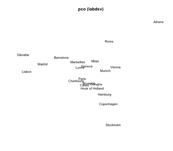

5) MDS with pcoa()

The package "ape" provides the function pcoa() (Principal Coordinates Analysis). Its general usage has the following form:

pcoa(D, correction="none", rn = NULL)

# 5) MDS 'pcoa'
mds5 = pcoa(eurodist)

# plot
plot(mds5$vectors[,1], mds5$vectors[,2], type = "n", xlab = "", ylab = "",
     axes = FALSE, main = "pcoa (ape)")
text(mds5$vectors[,1], mds5$vectors[,2], labels(eurodist), 
     cex = 0.9, xpd = TRUE)

6) MDS with dudi.pco()

The package "ade4" provides the function dudi.pco() (Principal Coordinates Analysis). Its general usage has the following form:

dudi.pco(d, row.w = "uniform", scannf = TRUE, nf = 2, full = FALSE, tol = 1e-07)

# 6) MDS 'dudi.pco'
mds6 = dudi.pco(eurodist, scannf = FALSE, nf = 2)

## Warning: Non euclidean distance

# plot
plot(mds6$li[,1], mds6$li[,2], type = "n", xlab = "", ylab = "",
     axes = FALSE, main = "dudi.pco (ade4)")
text(mds6$li[,1], mds6$li[,2], labels(eurodist), cex = 0.9)

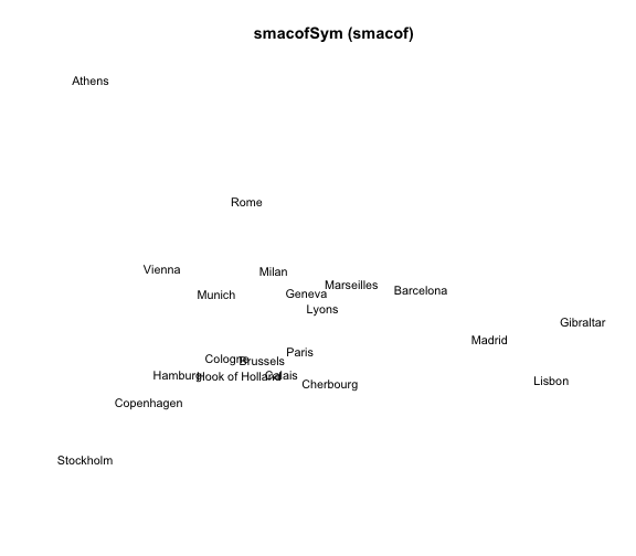
7) MDS with smacofSym()

The package "smacof" provides the function smacofSym() (Multidimensional scaling (stress minimization: SMACOF) on symmetric dissimilarity matrix.). This function uses a majorization approach to get the solution (more info in this ade4. Its general usage has the following form:

smacofSym(delta, ndim = 2, weightmat = NULL, init = NULL, metric = TRUE, ties = "primary", verbose = FALSE, relax = FALSE, modulus = 1, itmax = 1000, eps = 1e-06)

# 7) MDS 'smacofSym'
mds7 = smacofSym(eurodist, ndim = 2)

# plot
plot(mds7$conf[,1], mds7$conf[,2], type = "n", xlab = "", ylab = "",
     axes = FALSE, main = "smacofSym (smacof)")
text(mds7$conf[,1], mds7$conf[,2], labels(eurodist), 
     cex = 0.9, xpd = TRUE)