3 First Contact with R
If you are new to R and don’t have any programming experience, then you should read this chapter in its entirety. If you already have some previous experience working with R and/or have some programming background, then you may want to skim over most of the introductory chapters of part I.
This chapter, and the rest of the book, assumes that you have installed both R and RStudio in your computer. If this is not the case, then go to chapters Installing R and Installing RStudio to follow the steps for downloading and installing these programs.
R comes with a simple built-in graphical user interface (GUI), and you can certainly start working with it right out of the box. That is actually the way I got my first contact with R back in 2001 during my senior year in college. Nowadays, instead of using R’s GUI, it is more convenient to interact with R using a third party software such as RStudio.
I describe more introductory details about RStudio in the next chapter A Quick Tour Around RStudio. For now, go ahead and launch RStudio in your computer.
3.1 First Contact with R (via RStudio)
When you open RStudio, you should be able to see its layout organized into quadrants officially called panes. The very first time you launch RStudio you will only see three panes, like in the screenshot below.
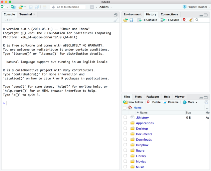
Figure 3.1: Screenshot of RStudio when launched for the first time.
To help you break the ice with R, it’s better if we start working directly on the Console.
As you can tell from the following screenshot, the console is located in the left-hand side quadrant of RStudio. Keep in mind that your RStudio’s console pane may be located in a different quadrant.
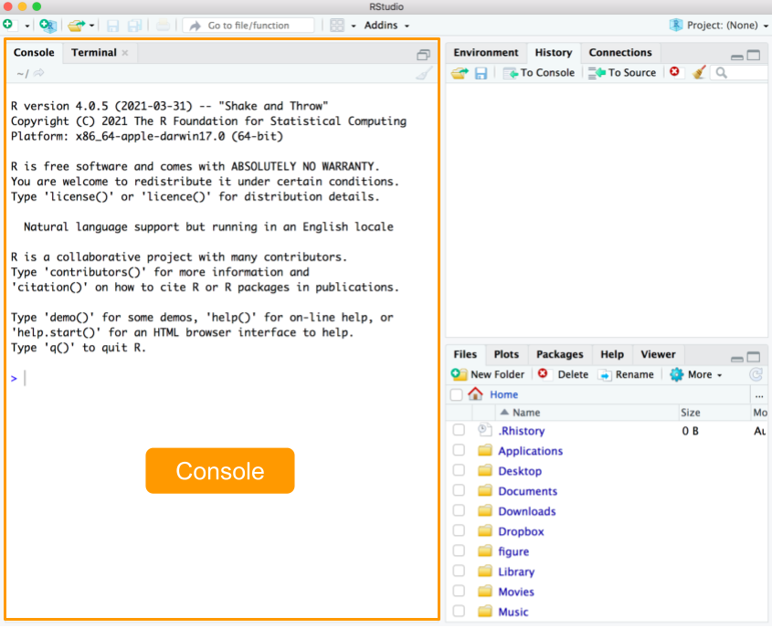
Figure 3.2: Console quadrant in RStudio.
Technically speaking, the console is a terminal where a user inputs commands and views output. Simply put, this is where you can directly interact with R by typing commands, and getting the output from the execution of the commands.
3.1.1 R as a scientific calculator
This first activity is dedicated for readers with little or no programming experience, especially those of you who have never used software in which you have to type commands. The idea is to start typing simple things in the console, basically using R as a scientific calculator.
Here’s a toy example. Consider the monthly bills of an undergraduate student:
- cell phone $80
- transportation $20
- groceries $527
- gym $10
- rent $1500
- other $83
You can use R to find the student’s total expenses by typing these commands in the console:
80 + 20 + 527 + 10 + 1500 + 83There is nothing surprising or fancy about this piece of code. In fact, it has
all the numbers and all the + symbols that you would use if you had to obtain
the total expenses by using the calculator in your cellphone.
3.1.2 Assigning values to objects
Often, it will be more convenient to create objects, sometimes also called
variables, that store one or more values. To do this, type the name of the
object, followed by the assignment or “arrow” operator <-, followed by the
assigned value. By the way, the arrow operator consists of a left-angle bracket
< (or “less than” symbol) and a dash or hyphen symbol -.
For example, you can create an object phone to store the value of the monthly
cell phone bill, and then inspect the object by typing its name:
phone <- 80
phone
> [1] 80
All R statements where you create objects are known as assignments, and they have this form:
object <- valuethis means you assign a value to a given object; one easy way to read the
previous assignment is “phone gets 80”.
Alternatively, you can also use the equals sign = for assignments:
transportation = 20
transportation
> [1] 20
As you will see in the rest of the book, I’ve written most assignments with the
arrow operator <-. But you can perfectly replace them with the equals sign
=. The opposite is not necessarily true. There are some especial cases in
which an equals sign cannot be replaced with the arrow, but we’ll talk about
this later.
Pro tip. RStudio has a keyboard shortcut for the arrow operator<-:
Windows & Linux users:
Alt+-Mac users:
Option+-
In fact, there is a large set of keyboard shortcuts. In the menu bar, go to the Help tab, and then click on the option Keyboard Shorcuts Help to find information about all the available shortcuts.
3.1.3 Object Names
There are certain rules you have to follow when creating objects and variables. Object names cannot start with a digit and cannot contain certain other characters such as a comma or a space.
The following are invalid names (and invalid assignments)
# cannot start with a number
5variable <- 5

# cannot start with an underscore
_invalid <- 10

# cannot contain comma
my,variable <- 3

# cannot contain spaces
my variable <- 1
People use different naming styles, and at some point you should also adopt a convention for naming things. Some of the common styles are:
snake_case

camelCase

period.case
Pretty much all the objects and variables that I create in this book follow the “snake_case” style. It is certainly possible that you may end up working with a team that has a style-guide with a specific naming convention. Feel free to try various styles, and once you feel comfortable with one of them, then stick to it.
3.1.4 Case Sensitive
R is case sensitive. This means that phone is not the same as Phone or
PHONE
# case sensitive
phone <- 80
Phone <- -80
PHONE <- 8000

phone + Phone
> [1] 0

PHONE - phone
> [1] 7920
Again, this is one more reason why adopting a naming convention early on in a data analysis or programming project is very important. Being consistent with your notation may save you from some headaches down the road.
3.1.5 Calling Functions
Like any other programming language, R has many functions. To use a function just type its name followed by parenthesis. Inside the parenthesis you typically pass one or more inputs. Most functions will produce some type of output:
# absolute value
abs(10)
abs(-4)

# square root
sqrt(9)

# natural logarithm
log(2)
In the above examples, the functions are taking a single input. But often you
will be working with functions that accept several inputs. The log() function
is one them. By default, log() computes the natural logarithm. But it also
has the base argument that allows you to specify the base of the logarithm,
say to base = 10
log(10, base = 10)
> [1] 13.2 Getting Help
Because we work with functions all the time, it’s important to know certain details about how to use them, what input(s) is required, and what is the returned output.
So how do you find all this information technically known as a function’s documentation? There are several ways to access this type of information.
If you know the name of a function you are interested in knowing more about,
you can use the function help() and pass it the name of the function you
are looking for:
# documentation about the 'abs' function
help(abs)

# documentation about the 'mean' function
help(mean)
Alternatively, you can use a shortcut using the question mark ? followed
by the name of the function:
# documentation about the 'abs' function
?abs

# documentation about the 'mean' function
?mean
help() and ? only work if you know the name of the function your are
looking for. Sometimes, however, you don’t know the name of the function but
you may know some keyword(s). To look for related functions associated to a
keyword, use help.search() or simply type double question marks ??
# search for 'absolute'
help.search("absolute")

# alternatively you can also search like this:
??absolute
Notice the use of quotes surrounding the input name inside help.search()
Often overlooked by beginners but extremely helpful is to understand the anatomy of the information displayed in the technical documentation. The content is typically organized into seven sections listed below (although sometimes there may be less or more sections)
- Title
- Description
- Usage of function
- Arguments
- Details
- See Also
- Examples
The three screenshots below show the “Help” or technical documentation of the
log() function. This information is in RStudio’s Help tab, located in the
pane that contains other tabs such as Files, Plots, Packages.
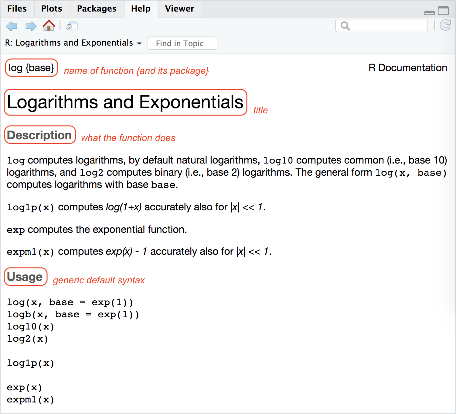
Figure 3.3: Help documentation for the log function (part 1)
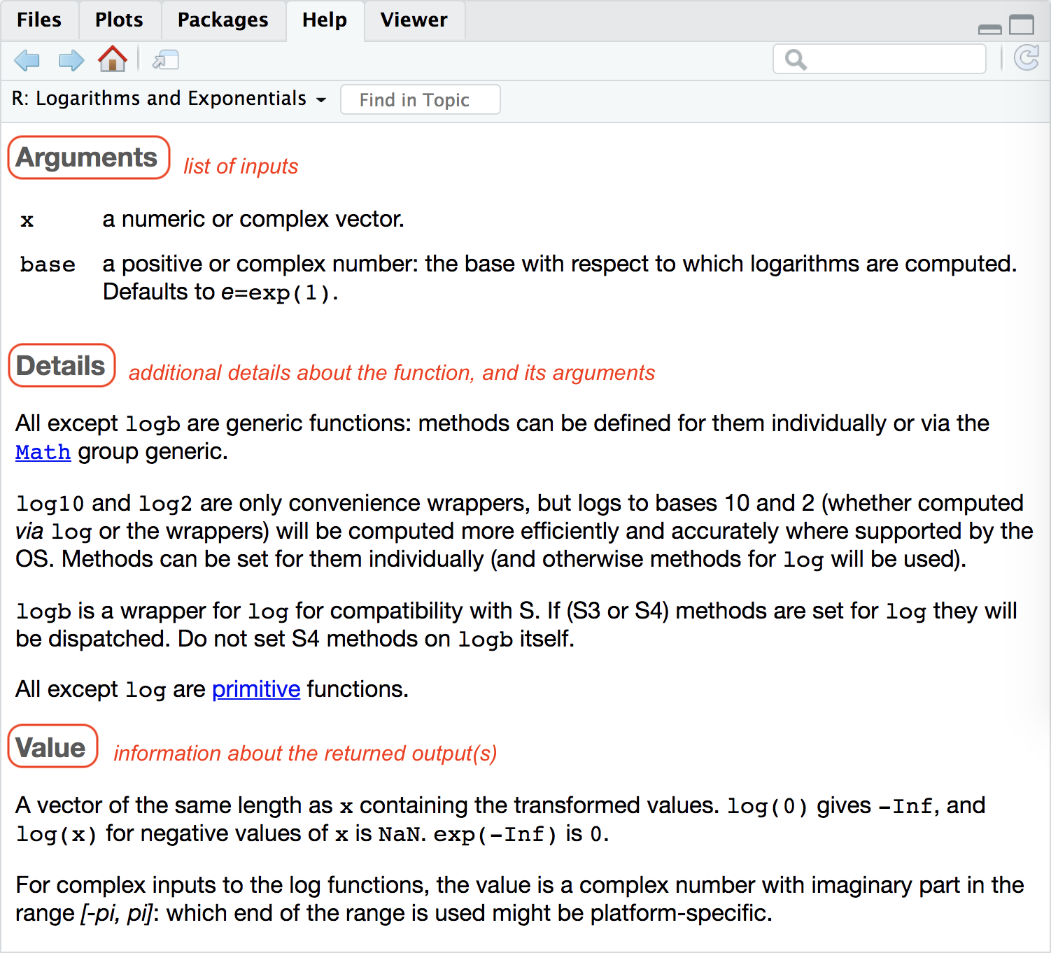
Figure 3.4: Help documentation for the log function (part 2)
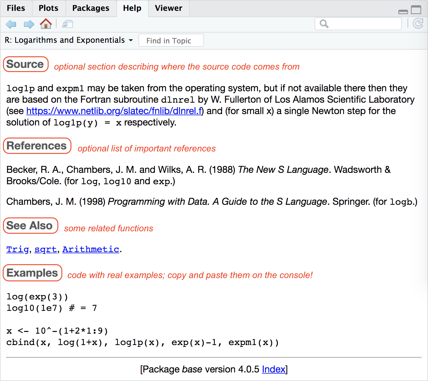
Figure 3.5: Help documentation for the log function (part 3)
3.3 Installing Packages
R comes with a large set of functions and packages. A package is a collection of functions that have been designed for a specific purpose. One of the great advantages of R is that many analysts, scientists, programmers, and users can create their own packages and make them available so that everybody can use them. R packages can be shared in different ways. The most common way to share a package is to submit it to what is known as CRAN, the Comprehensive R Archive Network.
You can install a package using the install.packages() function. To do this,
I recommend that you run this command directly on the console. In other
words, do not include this command in a source file (e.g. R script file, Rmd
file). The reason for running this command directly on the console is to avoid
getting an error message when running code from a source file.
To use install.packages() just give it the name of a package, surrounded by
quotes, and R will look for it in CRAN, and if it finds it, R will download it
to your computer.
# installing (run this on the console!)
install.packages("knitr")
You can also install a bunch of packages at once by placing their names,
each name separated by a comma, inside the c() function:
# run this command on the console!
install.packages(c("readr", "ggplot2"))
Once you installed a package, you can start using its functions by loading
the package with the function library(). For better or worse, library()
allows you to specify the name of the package with or without quotes. Unlike
install.packages() you can only specify the name of one package in library()
# (this command can be included in an Rmd file)
library(knitr)      # without quotes
library("ggplot2")  # with quotes
By the way, you only need to install a package once. After a package has been
installed in your computer, the only command that you need to invoke in order
to use its functions is the library() function.
3.4 Exercises
1) Here’s the list of monthly expenses for a hypothetical undergraduate student
- cell phone $80
- transportation $20
- groceries $550
- gym $15
- rent $1500
- other $83
Using the
consolepane of RStudio, create objects (i.e. variables) for each of these expenses listed above, and then create an objecttotalwith the sum of the expenses.Assuming that the student has the same expenses every month, how much would she spend during a school “semester”? (assume the semester involves five months). Write code in R to find this value.
Using the same assumption about the monthly expenses, how much would she spend during a school “year”? (assume the academic year is 10 months). Write code in R to find this value.
2) Use the function install.packages() to install packages "stringr",
"RColorBrewer", and "bookdown"
3) Write code in the console to calculate: \(3x^2 + 4x + 8\) when \(x = 2\)
4) Calculate: \(3x^2 + 4x + 8\) but now with a numeric sequence for \(x\)
using x <- -3:3
5) Find out how to look for information about math binary operators
like + or ^ (without using ?Arithmetic). Tip: quotes are your friend.
3.1.6 Comments in R
All programming languages use a set of characters to indicate that a specifc part or lines of code are comments, that is, things that are not to be executed. R uses the hash or pound symbol
#to specify comments. Any code to the right of#will not be executed by R.You will notice that I have included comments in almost all of the code snippets shown in the book. To be honest, some examples may have too many comments, but I’ve done that to be very explicit, and so that those of you who lack coding experience understand what’s going on. In real life, programmers use comments, but not so much as I do in the book. The main purpose of writing comments is to describe—conceptually—what is happening with certain lines of code. Some would even argue that comments should only be used to express not the what but the why a developer is doing something. In case of doubt, especially if you don’t have a lot of programming experience, I think it’s better to err on the side of caution by adding more comments than including no comments whatsoever.