ibtracs = st_read("IBTrACS.NA.list.v04r00.points")21 Shapefile Data
In this chapter we’ll work with geospatial data in shapefile format which is perhaps the most common format of geospatial vector data.
The code in this chapter requires the following packages:
library(tidyverse)      # data wrangling and graphics
library(lubridate)      # for working with dates
library(sf)             # for working with geospatial vector-data
library(rnaturalearth)  # maps data (e.g. US States)
library(leaflet)        # web interactive maps
21.1 Geospatial Data in Shapefile Format
Like in the previous lectures, we will work again with data about tropical cyclones in the North Atlantic. This time, however, instead of using the storms tibble from "dplyr", we will work with data from the International Best Track Archive for Climate Stewardship (IBTrACS).
21.1.1 What is a shapefile?
A shapefile is one particular file format to store geospatial vector data.
It’s a common standard for handling vector data.
It’s developed by ESRI as a mostly open format for GIS software products (e.g. ArcGIS).
Confusingly, a shapefile is NOT a single file, but a set of files.
21.1.2 What files are in a shapefile?
There are 3 core files to have at a minimum for a shapefile:
.shp stores the feature geometry (e.g. points, lines, polygons).
.dbf stores attributes information.
.shx index (i.e. link) between .shp and .dbf files.
Usually, although not always, there are other files:
.prj stores coordinate system information; used by ArcGIS.
.xml metadata in XML format about the shapefile.
.cpg codepage for identifying the characterset to be used.
21.2 IBTrACS Data
We are going to use data from the International Best Track Archive for Climate Stewardship or IBTrACS for short. IBTrACS is the most complete global collection of tropical cyclones available, and it is developed collaboratively with all the World Meteorological Organization (WMO) Regional Specialized Meteorological Centres, as well as other organizations and individuals from around the world.

21.2.1 Downloading Shapefiles
IBTrACS data sets come is various formats. We’ll use their data sets in shapefile format, available at:

For illustration purposes we’ll use data from the North Atlantic. To be more precise, we’ll work with the points geometry shapefile:
IBTrACS.NA.list.v04r00.points.zip: the geometries are points (i.e. points indicating the location of the storms)
21.2.2 Importing Shapefile Data
Assuming that the shapefile is in your working directory, and also that it has been decompressed, to import the data in R you use the "sf" function st_read():
Reading layer `IBTrACS.NA.list.v04r00.points' from data source
  `/Users/gaston/Library/CloudStorage/Dropbox/R-tidy-hurricanes/tidyhurricanes-quarto/data/IBTrACS.NA.list.v04r00.points'
  using driver `ESRI Shapefile'
Simple feature collection with 127171 features and 168 fields
Geometry type: POINT
Dimension:     XY
Bounding box:  xmin: -136.9 ymin: 7 xmax: 63 ymax: 83.01
Geodetic CRS:  WGS 84
It turns out that ibtracs is an sf object, and also a data.frame.
# what kind of object is ibtracs?
class(ibtracs)
[1] "sf" "data.frame"This means we can manipulate it like any other data table in R (e.g. with dplyr commands). For example, the first 15 attributes (columns) are:
# a few column names (of attributes)
names(ibtracs)[1:15]
[1] "SID" "SEASON" "NUMBER" "BASIN" "SUBBASIN"
[6] "NAME" "ISO_TIME" "NATURE" "LAT" "LON"
[11] "WMO_WIND" "WMO_PRES" "WMO_AGENCY" "TRACK_TYPE" "DIST2LAND" For convenience purposes, let’s select the first 12 columns:
ibtracs = select(ibtracs, 1:12)21.3 Maps with "ggplot2"
Like we did in the previous lectures, let’s see how to make plots with "ggplot2", "sf", and "rnaturalearth".
world_map = ne_countries(returnclass = "sf")21.3.1 Map of Storms in 1975 (1st attempt)
Notice that geom_sf() already understands that ibtracs, and ibtracs_1975 by extension, are data sets in a standard vector format. This means that we don’t need to specify anything for x and y axes. Isn’t that cool?
ibtracs_1975 = ibtracs |>
  filter(SEASON == 1975)

ggplot() +
  # country polygons
  geom_sf(data = world_map, fill = "beige") +
  # storms
  geom_sf(data = ibtracs_1975) +
  coord_sf(xlim = c(-110, 0), ylim = c(0, 60))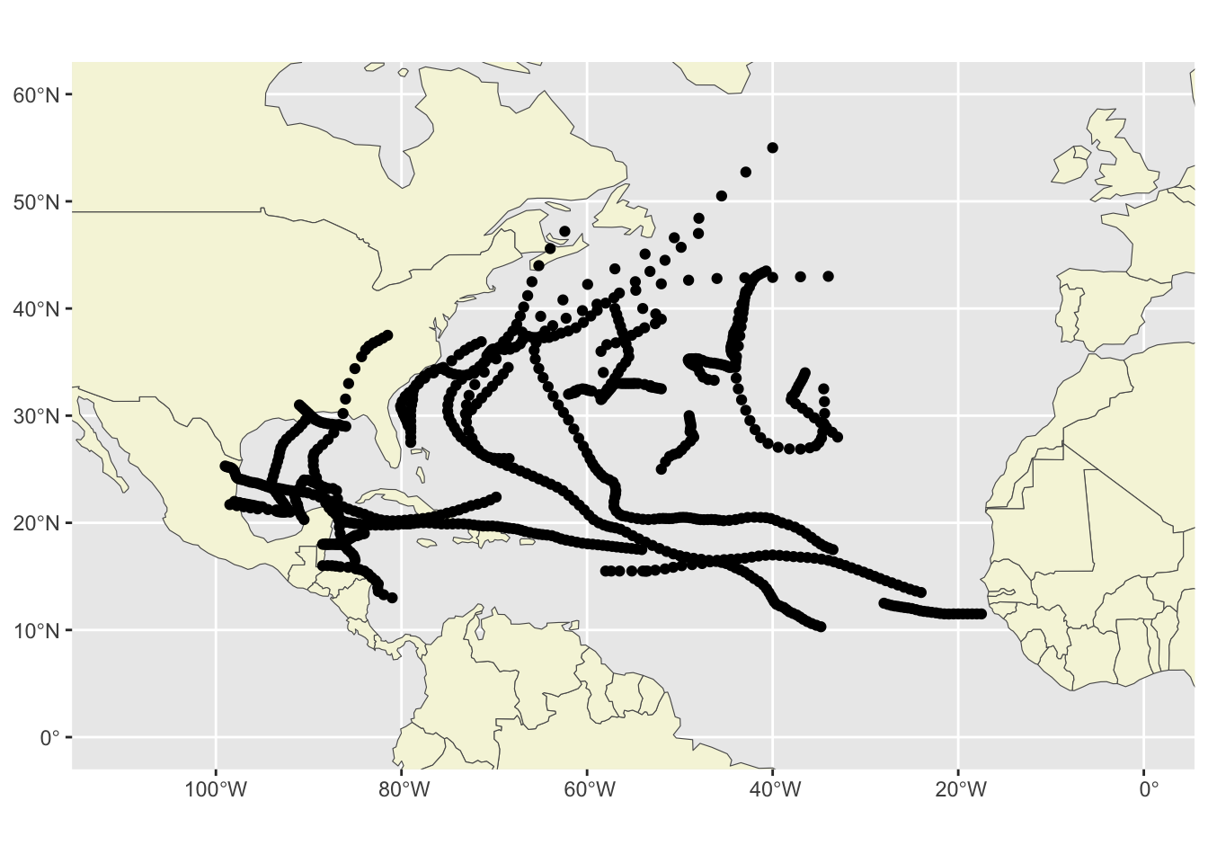
Notice that IBTrACS data has many more tropical cyclones than those in storms. Why? Because IBTrACS contains systems of low wind speed (i.e. baby storms that never became big enough to be named).
21.3.2 Map of Storms in 1975 (2nd attempt)
ggplot() +
  # country polygons
  geom_sf(data = world_map, fill = "beige") +
  # storms
  geom_sf(data = ibtracs_1975, aes(color = NATURE), linewidth = 1) +
  coord_sf(xlim = c(-110, 0), ylim = c(0, 60))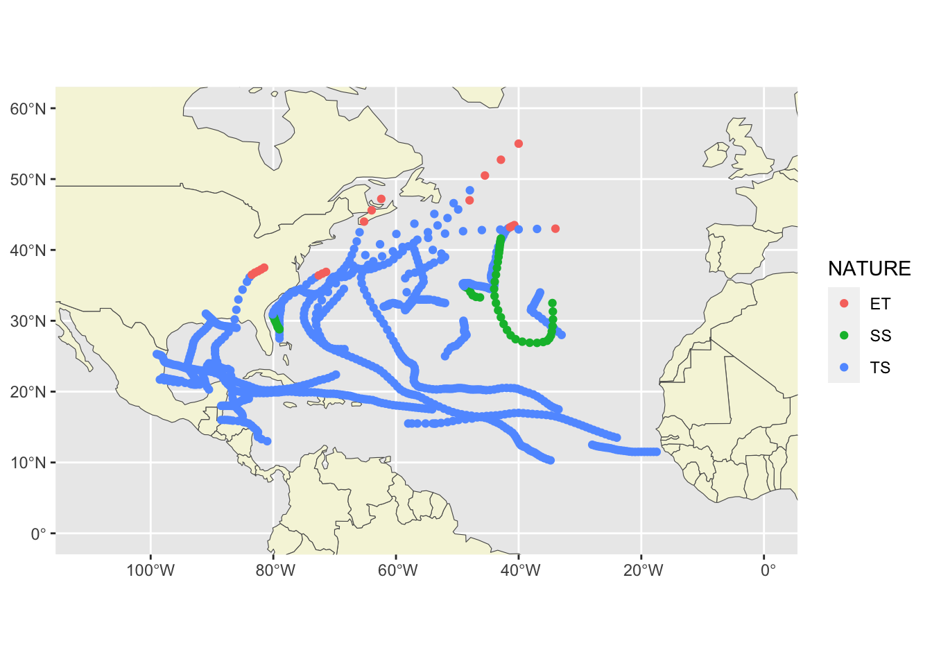
Again, if you want to know about the categories in column NATURE, please refer to the data documentation:
https://www.ncei.noaa.gov/sites/default/files/2021-07/IBTrACS_v04_column_documentation.pdf
21.4 Maps with "leaflet"
Let’s repeat the same tasks of section 3 but now making maps with "leaflet".
21.4.1 Plotting Storms in 1975
Starting from scratch, to visualize tropical cyclones from 1975 we subset ibtracs data for that year:
ibtracs_1975 = ibtracs |>
  filter(SEASON == 1975)
Then, we can pass this table to leaflet(), adding the addCircles() layer. Notice that ibtracs, and ibtracs_1975 by extension, already come in the appropriate format so that leaflet() knows which attributes to use for the lng and lat coordinates.
leaflet(data = ibtracs_1975) |>
  addTiles() |>
  addCircles(
    label = ~NAME
  )
21.4.2 Plotting Hurricanes in 1975
Instead of plotting all the storms in 1975, let’s plot only those that became hurricanes. To display the full trajectory of the hurricanes we need to do some filtering and data manipulation:
# tropical cyclones in 1975,
# selecting first 12 columns
ibtracs_1975 = ibtracs |>
  filter(SEASON == 1975) |>
  select(1:12)

# auxiliary table with names of hurricanes
# winds of 6 knots or greater (to identify hurricanes)
hurricane_names_1975 = ibtracs_1975 |>
  filter(WMO_WIND >= 65) |>
  distinct(NAME)

# generate color for each storm
hurricane_names_1975$COLOR = rainbow(n = nrow(hurricane_names_1975))

# merge colors
hurricanes_1975 = inner_join(ibtracs_1975, hurricane_names_1975, by = "NAME")
# map of hurricanes in 1975,
# color coding by NAME, and taking ISO_WID into account
leaflet(data = hurricanes_1975) |>
addTiles() |>
addCircles(
label = ~NAME,
color = ~COLOR,
weight = ~WMO_WIND/10
)