8 Basic Manipulation Examples

8.1 Introduction

This chapter provides more elaborated examples than the simple demos presented so far. The idea is to show you less abstract scenarios and cases where you could apply the functions and concepts covered so far.

8.1.1 Example: Names of files

Imagine that you need to generate the names of 10 data .csv files. All the files have the same prefix name but each of them has a different number: file1.csv, file2.csv, … , file10.csv.

There are several ways in which you could generate a character vector with these names. One naive option is to manually type those names and form a vector with c()

c('file1.csv', 'file2.csv', 'file3.csv')
#> [1] "file1.csv" "file2.csv" "file3.csv"

But that’s not very efficient. Just think about the time it would take you to create a vector with 100 files. A better alternative is to use the vectorized nature of paste()

paste('file', 1:10, '.csv', sep = "")
#>  [1] "file1.csv"  "file2.csv"  "file3.csv"  "file4.csv"  "file5.csv" 
#>  [6] "file6.csv"  "file7.csv"  "file8.csv"  "file9.csv"  "file10.csv"

Or similarly with paste0()

paste0('file', 1:10, '.csv')
#>  [1] "file1.csv"  "file2.csv"  "file3.csv"  "file4.csv"  "file5.csv" 
#>  [6] "file6.csv"  "file7.csv"  "file8.csv"  "file9.csv"  "file10.csv"

8.1.2 Example: Valid Color Names

R comes with the function colors() that returns a vector with the names (in English) of 657 colors available in R. How would you write a function is_color() to test if a given name—in English—is a valid R color. If the provided name is a valid R color, is_color() should return TRUE. If the provided name is not a valid R color is_color() should return FALSE.

is_color <- function(x) {
  x %in% colors()
}

Lets test it:

is_color('yellow')  # TRUE
#> [1] TRUE

is_color('blu')     # FALSE
#> [1] FALSE

is_color('turkuiose') # FALSE
#> [1] FALSE

Another possible way to write is_color() is comparing if any() element of colors() equals the provided name:

is_color2 <- function(x) {
  any(colors() == x)
}

Test it:

is_color2('yellow')  # TRUE
#> [1] TRUE

is_color2('blu')     # FALSE
#> [1] FALSE

is_color2('turkuiose') # FALSE
#> [1] FALSE

8.1.3 Example: Me and You plot

This example is not really about data analysis or something serious, it is instead a fun project in which you get to apply what we have covered so far. The idea is to produce a plot with some text on it. But not any kind of text. The plot is intended to be a postcard—for Saint Valentine’s day. With this kind of tutorial, you should be able to make youw own plot, print it and give it to your significant other.

The idea is to make a chart with your name and the name of your significant other, adding a touch of randomness in the location of the text, the sizes, and the colors.

First we generate the x-y coordinates. We’ll use 100 points, and set the random seed to 333:

# random seed
set.seed(333)

# x-y coordinates
n <- 100
x <- rnorm(n)
y <- rnorm(n, 1, 2)

The first step is to produce a very basic-raw plot (nothing fancy). We use plot() for this purpose:

plot(x, y)

This just produces a scatter diagram with a 100 points on it. The following step consists of replacing the dots by some text: your name and the one of your significant other. To hide the dots, we set the parameter type = "n", which means that we don’t want anything to be plotted. To show the text, we use the low level plotting function text(). We use the same coordinates, but this time we specify the displayed labels:

plot(x, y, type = "n")
text(x, y, labels = "me & you")

Again, this is a very preliminary plot; something basic that allows us to start getting a feeling of how the chart looks like. The second step is to change the background color. One way to do this is by specifying the bg graphical parameter inside the par() function:

# graphical parameters
op <- par(bg = "gray10")
# plot text
plot(x, y, type = "n")
text(x, y, 
     labels = "me & you",
     col = "white")
# reset default parameters
par(op)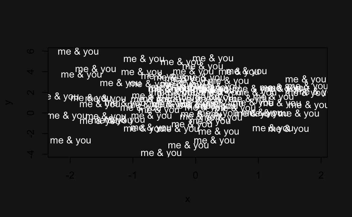

par() has default settings. Everytime you call par() and change one of the associated parameters, the subsequent plots will be displayed with those values. To set parameters in a temporary way, you can assign them to an object: i.e. op. After the plot is produced, we reset the default graphical parameters with the instruction par(op).

We are getting closer to the desired look of the postcard. The final stage is to add some color to the text, and change their size. The size of the labels will also be random with a uniform distribution.

R provides several ways to specify colors. In this example we will use the hsv() function (i.e. hue-saturation-value). This function requires three parameters: hue (color), saturation, and value. Hues are specified with a range from 0 to 1. We generate some random numbers in the interval 0.85 - 0.95 to get some hues red, pink, fuchsia colors. hsv() also takes the optional parameters alpha to determined the alpha transparency.

# text size
sizes <- runif(n, 0.5, 3)

# text color
hues <- runif(n, 0.85, 0.95)
alphas <- runif(n, 0.1, 1)


op <- par(bg = "gray10", mar = rep(0, 4))
plot(x, y, type = "n", axes = FALSE, 
     xlab = '', ylab = '')
text(x, y, 
     labels = "me & you", 
     font = 3, 
     col = hsv(hues, 1, 1, alphas),
     cex = sizes)
par(op)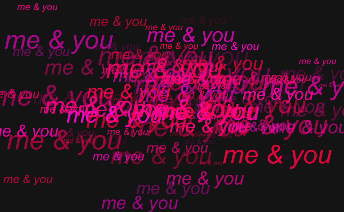

To save the image, call pdf(). To give the image the dimensions of a standard postcard, you can specify width = 5 and height = 3.5, that is, 5 inches wide and 3.5 inches tall (you can choose other dimensions if you want):

pdf(file = "figure/me-and-you3.pdf", width = 5, height = 3.5)
op <- par(bg = "gray10", 
          mar = rep(0, 4))
plot(x, y, type = "n", axes = FALSE, 
     xlab = '', ylab = '')
text(x, y, 
     labels = "me & you", 
     font = 3, 
     col = hsv(hues, 1, 1, alphas),
     cex = sizes)
par(op)
dev.off()

If you save the image in png format, you could also use it as a wallpaper for your computer:

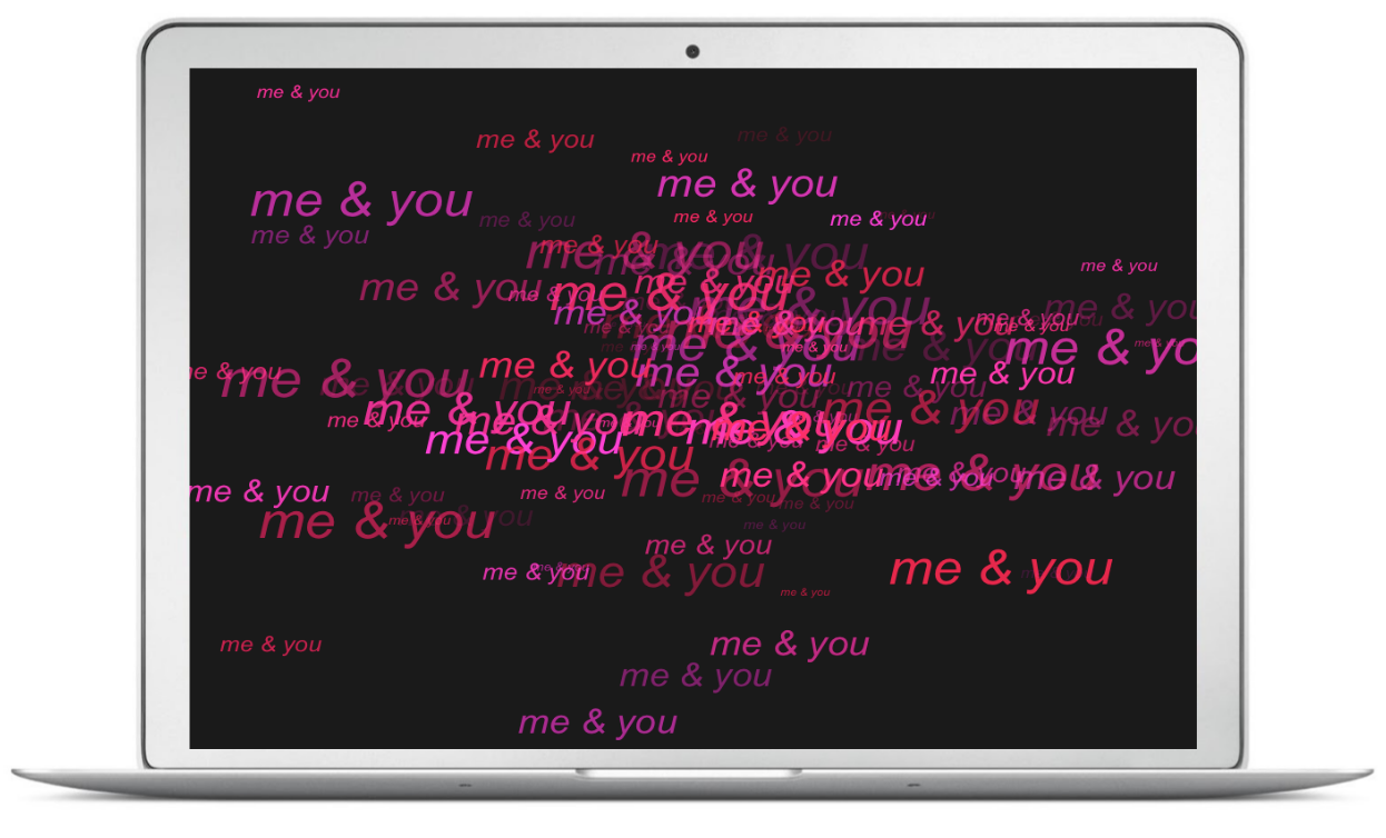
A wallpaper chart for your significant other

---

Make a donation

If you find this resource useful, please consider making a one-time donation in any amount. Your support really matters.