21 BMC Journals Data

library(stringr)

21.1 Introduction

In this example we will work analyzing some text data. We will analyze an old catalog of journals from the BioMed Central (BMC), a scientific publisher that specializes in open access journal publication. You can find more informaiton of BMC at: https://www.biomedcentral.com/journals

The data with the journal catalog is no longer available at BioMed’s website, but you can find a copy in the book’s github repository:

https://raw.githubusercontent.com/gastonstat/r4strings/master/data/biomedcentral.txt

To download a copy of the text file to your working directory, run the following code:

# download file
github <- "https://raw.githubusercontent.com/gastonstat/r4strings"
textfile <- "/master/data/biomedcentral.txt"
download.file(url = paste0(github, textfile), destfile = "biomedcentral.txt")

To import the data in R you can read the file with read.table():

# read data (stringsAsFactors=FALSE)
biomed <- read.table('biomedcentral.txt', header = TRUE, stringsAsFactors = FALSE)

You can check the structure of the data with the function str():

# structure of the dataset
utils::str(biomed, vec.len = 1)
#> 'data.frame':    336 obs. of  7 variables:
#>  $ Publisher     : chr  "BioMed Central Ltd" ...
#>  $ Journal.name  : chr  "AIDS Research and Therapy" ...
#>  $ Abbreviation  : chr  "AIDS Res Ther" ...
#>  $ ISSN          : chr  "1742-6405" ...
#>  $ URL           : chr  "http://www.aidsrestherapy.com" ...
#>  $ Start.Date    : int  2004 2011 ...
#>  $ Citation.Style: chr  "BIOMEDCENTRAL" ...

As you can see, the data frame biomed has 336 observations and 7 variables. Actually, all the variables except for Start.Date are in character mode.

21.2 Analyzing Journal Names

We will do a simple analysis of the journal names. The goal is to study what are the more common terms used in the title of the journals. We are going to keep things at a basic level but for a more formal (and sophisticated) analysis you can check the package tm —text mining— (by Ingo Feinerer).

To have a better idea of what the data looks like, let’s check the first journal names.

# first 5 journal names
head(biomed$Journal.name, n = 5)
#> [1] "AIDS Research and Therapy"            
#> [2] "AMB Express"                          
#> [3] "Acta Neuropathologica Communications" 
#> [4] "Acta Veterinaria Scandinavica"        
#> [5] "Addiction Science & Clinical Practice"

As you can tell, the fifth journal "Addiction Science & Clinical Practice" has an ampersand & symbol. Whether to keep the ampersand and other punctutation symbols depends on the objectives of the analysis. In our case, we will remove those elements.

21.2.1 Preprocessing

The preprocessing steps implies to get rid of the punctuation symbols. For convenience, I recommended that you start working with a small subset of the data. In this way you can experiment at a small scale until we are confident with the right manipulations. Let’s take the first 10 journals:

# get first 10 names
titles10a <- biomed$Journal.name[1:10]
titles10a
#>  [1] "AIDS Research and Therapy"            
#>  [2] "AMB Express"                          
#>  [3] "Acta Neuropathologica Communications" 
#>  [4] "Acta Veterinaria Scandinavica"        
#>  [5] "Addiction Science & Clinical Practice"
#>  [6] "Agriculture & Food Security"          
#>  [7] "Algorithms for Molecular Biology"     
#>  [8] "Allergy, Asthma & Clinical Immunology"
#>  [9] "Alzheimer's Research & Therapy"       
#> [10] "Animal Biotelemetry"

We want to get rid of the ampersand signs &, as well as other punctuation marks. This can be done with str_replace_all() and replacing the pattern [[:punct:]] with empty strings "" (don’t forget to load the "stringr" package)

# remove punctuation
titles10b <- str_replace_all(titles10a, pattern = "[[:punct:]]", "")
titles10b
#>  [1] "AIDS Research and Therapy"           
#>  [2] "AMB Express"                         
#>  [3] "Acta Neuropathologica Communications"
#>  [4] "Acta Veterinaria Scandinavica"       
#>  [5] "Addiction Science  Clinical Practice"
#>  [6] "Agriculture  Food Security"          
#>  [7] "Algorithms for Molecular Biology"    
#>  [8] "Allergy Asthma  Clinical Immunology" 
#>  [9] "Alzheimers Research  Therapy"        
#> [10] "Animal Biotelemetry"

We succesfully replaced the punctuation symbols with empty strings, but now we have extra whitespaces. To remove the whitespaces we will use again str_replace_all() to replace any one or more whitespaces
\\s+ with a single blank space " ".

# trim extra whitespaces
titles10c <- str_replace_all(titles10b, pattern = "\\s+", " ")
titles10c
#>  [1] "AIDS Research and Therapy"           
#>  [2] "AMB Express"                         
#>  [3] "Acta Neuropathologica Communications"
#>  [4] "Acta Veterinaria Scandinavica"       
#>  [5] "Addiction Science Clinical Practice" 
#>  [6] "Agriculture Food Security"           
#>  [7] "Algorithms for Molecular Biology"    
#>  [8] "Allergy Asthma Clinical Immunology"  
#>  [9] "Alzheimers Research Therapy"         
#> [10] "Animal Biotelemetry"

Once we have a better idea of how to preprocess the journal names, we can proceed with all the 336 titles.

# remove punctuation symbols
all_titles <- str_replace_all(biomed$Journal.name, pattern = "[[:punct:]]", "")

# trim extra whitespaces
all_titles <- str_replace_all(all_titles, pattern = "\\s+", " ")

The next step is to split up the titles into its different terms (the output is a list).

# split titles by words
all_titles_list <- str_split(all_titles, pattern = " ")

# show first 2 elements
all_titles_list[1:2]
#> [[1]]
#> [1] "AIDS"     "Research" "and"      "Therapy" 
#> 
#> [[2]]
#> [1] "AMB"     "Express"

21.3 Summary statistics

So far we have a list that contains the words of each journal name. Wouldn’t be interesting to know more about the distribution of the number of terms in each title? This means that we need to calculate how many words are in each title. To get these numbers let’s use length() within sapply(); and then let’s tabulate the obtained frequencies:

# how many words per title
words_per_title <- sapply(all_titles_list, length)

# table of frequencies
table(words_per_title)
#> words_per_title
#>   1   2   3   4   5   6   7   8   9 
#>  17 108  81  55  33  31   6   4   1

We can also express the distribution as percentages, and we can get some summary statistics with summary()

# distribution
100 * round(table(words_per_title) / length(words_per_title), 4)
#> words_per_title
#>     1     2     3     4     5     6     7     8     9 
#>  5.06 32.14 24.11 16.37  9.82  9.23  1.79  1.19  0.30

# summary
summary(words_per_title)
#>    Min. 1st Qu.  Median    Mean 3rd Qu.    Max. 
#>    1.00    2.00    3.00    3.36    4.00    9.00

Looking at summary statistics we can say that around 30% of journal names have 2 words. Likewise, the median number of words per title is 3 words.

Interestingly the maximum value is 9 words. What is the journal with 9 terms in its title? We can find the longest journal name as follows:

# longest journal
all_titles[which(words_per_title == 9)]
#> [1] "Journal of Venomous Animals and Toxins including Tropical Diseases"

21.4 Common words

Remember that our main goal with this example is to find out what words are the most common in the journal titles. To answer this question we first need to create something like a dictionary of words. How do get such dictionary? Easy, we just have to obtain a vector containing all the words in the titles:

# vector of words in titles
title_words <- unlist(all_titles_list)

# get unique words
unique_words <- unique(title_words)

# how many unique words in total
num_unique_words <- length(unique(title_words))
num_unique_words
#> [1] 441

Applying unique() to the vector title_words we get the desired dictionary of terms, which has a total of 441 words.

Once we have the unique words, we need to count how many times each of them appears in the titles. Here’s a way to do that:

# vector to store counts
count_words <- rep(0, num_unique_words)

# count number of occurrences
for (i in 1:num_unique_words) {
  count_words[i] <- sum(title_words == unique_words[i])
}

An alternative simpler way to count the number of word occurrences is by using the table() function on title\_words:

# table with word frequencies
count_words_alt <- table(title_words)

In any of both cases (count_words or count_words_alt), we can examine the obtained frequencies with a simple table:

# table of frequencies
table(count_words)
#> count_words
#>   1   2   3   4   5   6   7   9  10  12  13  16  22  24  28  30  65  67  83  86 
#> 318  61  24   8   5   7   1   2   2   2   1   2   1   1   1   1   1   1   1   1

# equivalently
table(count_words_alt)
#> count_words_alt
#>   1   2   3   4   5   6   7   9  10  12  13  16  22  24  28  30  65  67  83  86 
#> 318  61  24   8   5   7   1   2   2   2   1   2   1   1   1   1   1   1   1   1

21.5 The top 30 words

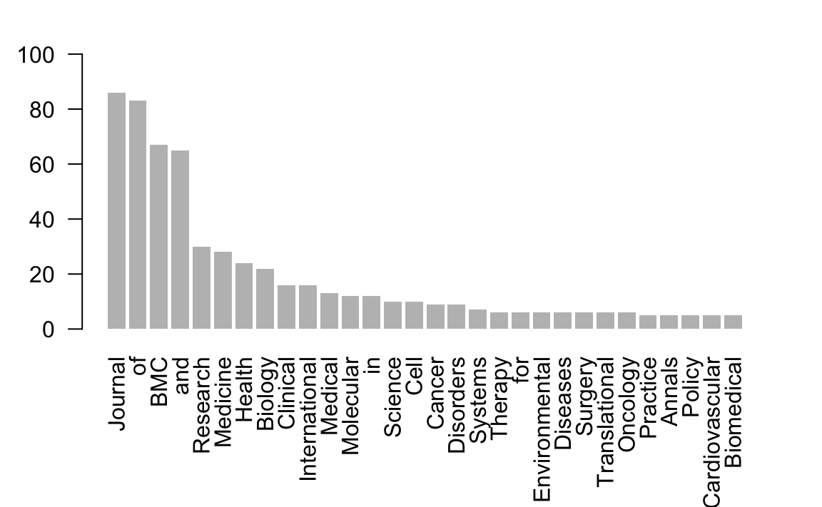
For illustration purposes let’s examine which are the top 30 common words.

# index values in decreasing order
top_30_order <- order(count_words, decreasing=TRUE)[1:30]

# top 30 frequencies
top_30_freqs <- sort(count_words, decreasing=TRUE)[1:30]

# select top 30 words
top_30_words <- unique_words[top_30_order]
top_30_words
#>  [1] "Journal"        "of"             "BMC"            "and"           
#>  [5] "Research"       "Medicine"       "Health"         "Biology"       
#>  [9] "Clinical"       "International"  "Medical"        "Molecular"     
#> [13] "in"             "Science"        "Cell"           "Cancer"        
#> [17] "Disorders"      "Systems"        "Therapy"        "for"           
#> [21] "Environmental"  "Diseases"       "Surgery"        "Translational" 
#> [25] "Oncology"       "Practice"       "Annals"         "Policy"        
#> [29] "Cardiovascular" "Biomedical"

To visualize the top_30_words we can plot them with a barchart using barplot():

# barplot
barplot(top_30_freqs, 
        border = NA, 
        names.arg = top_30_words, 
        las = 2, 
        ylim = c(0,100))

---

Make a donation

If you find this resource useful, please consider making a one-time donation in any amount. Your support really matters.