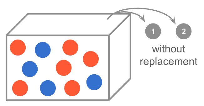
Consider a box containing 10 balls: 4 blue and 6 red, as displayed in the following figure. Assume you pick a 1st ball, then a 2nd ball (no replacement).
Refer to the box of the preceding problem. The following code allows you to simulate drawing 2 balls from the box 100 times—via replicate(). In order to use tidyverse functions, we need to reshape the simulations output into a data.frame.
  first second
1   red    red
2   red   blue
3  blue    red
4   red   blue
5  blue    red
6   red    red
Examples
Say we want to approximate probability of getting a first blue ball.
# proportion: 1st ball is blueballs_df |>summarize(prop_1blue =mean(first =="blue"))
  prop_1blue
1       0.44
What if we we want to approximate probability of getting the first ball blue, and the second ball red?
# proportion: 1st is blue, 2nd is redballs_df |>summarize(prop_1blue_2red =mean(first =="blue"& second =="red"))
  prop_1blue_2red
1             0.3
Your Turn
Change the value of set.seed() and increase the number of simulations to 1000. Write R pipelines to approximate the following probabilities. How do these approximations compare to the probabilities you calculated?
Approximate the probability that both balls are blue.
Show answer
balls_df |>summarize(mean(first =="blue"& second =="blue"))
Approximate the probability that 1st ball is red, 2nd ball is blue.
Show answer
# b) 1st is red, 2nd is blueballs_df |>summarize(mean(first =="red"& second =="blue"))
Approximate the probability that both balls are red.
Show answer
# c) both are redballs_df |>summarize(mean(first =="red"& second =="red"))
Approximate the probability 1st ball is blue or 2nd ball is blue.
Show answer
# d) 1st is blue OR 2nd is blueballs_df |>summarize(mean(first =="blue"| second =="blue"))
Approximate the probability 2nd ball is blue, given 1st ball is red.
Show answer
# e) 2nd is blue, given that 1st is redballs_df |>filter(first =="red") |>summarize(mean(second =="blue"))
Approximate the probability 2nd ball is blue, given 1st ball is blue.
Show answer
# f) 2nd is blue, given that 1st is blueballs_df |>filter(first =="blue") |>summarize(mean(second =="blue"))
Approximate the probability 1st ball is blue, given 2nd ball is red.
Show answer
# g) 1st is blue, given that 2nd is redballs_df |>filter(second =="red") |>summarize(mean(first =="blue"))
3) Students in STAT 101
Suppose that 35% of students in STAT 101 are from Southern California, 40% are from Northern California, and 25% are from outside California. What is the probability that a student selected at random:
Will be from Southern CA?
Will not be from Northern CA?
Will be from Southern or Northern CA?
Will be from Northern California, given that they are not from Southern CA?
Will be from Northern California, given that they are not from outside CA?
Show answers
0.35
0.35 + 0.25 = 0.6
0.35 + 0.40 = 0.75
0.4 / 0.65
0.4 / 0.75
5) Tickets from a box
Suppose we draw 2 tickets at random without replacement from a box with tickets marked {1, 2, 3, . . . , 9}. Find the probability that:
The first ticket drawn is labeled with an even number.
The second ticket drawn is labeled with an even number.
Both tickets drawn are labeled with an even number.
At least one of the tickets drawn is labeled with an even number.
The first ticket drawn is labeled with a prime number (recall that 1 is not a prime).
The second ticket drawn is labeled with a prime number.
Both tickets drawn are labeled with a prime number.
At least one of the tickets drawn is labeled with a prime number.
Show answers
(32/72) = 4/9
(32/72) = 4/9
(4/9) (3/8) = 12/72
P(at least one even) = 1 - P(none are even) = 1 - (5/9)(4/8) = 52/72
(32/72) = 4/9
(32/72) = 4/9
(4/9) (3/8) = 12/72
P(at least one prime) = 1 - P(none are prime) = 1 - (5/9)(4/8) = 52/72
6) Matching Probabilities
Match the terms (a-f) with their definitions (i-vi)
Terms
P(A|B) = P(A and B) / P(B)
P(A or B) = P(A) + P(B) - P(A and B)
P(A|B) = P(A)
P(A) = P(B)
P(A and B) = P(B | A) P(A)
P(A and B) = 0
Definitions
equally likely
mutually exclusive
conditional probability
multiplication rule
independence
addition rule
Show answers
with (d)
with (f)
with (a)
with (e)
with (c)
with (b)
7) Roll a pair of dice
You roll a red die and a blue die, both fair and independent. Find the probability that:
The red die and the blue die both roll 1’s.
The red die and the blue die both roll the same number.
The number on the red die is bigger than the one on the blue die.
The red die rolls a 3.
At least one die rolls a 3.
Exactly one die rolls a 3.
The smallest number on either die is 4.
The largest number on either die is 4.
At least one of the dice rolls a number greater than 4.
Exactly one of the dice rolls a number greater than 4.
The numbers on the dice sum to 7.
The numbers on the dice sum to 4.
Show answers
1/36
1/6
15/36
1/6
11/36
10/36
5/36
7/36
20/36
16/36
6/36
3/36
8) Students’ Club
A students’ club has 90 members. Fifty are Statistics majors and fifty are Applied Math (A.M.) majors. There are some that are double majoring in Stats and A.M. What is the probability that a member selected at random:
Is a double major?
Is a Stats major but not an A.M. major?
Is an A.M. major but not a Stats major?
Show answers
10/90
40/90
40/90
9) Finding probabilities
Suppose that A and B are independent events with \(P(A)\) = 0.7, and \(P(B^c)\) = 0.4. Find the following probabilities: