Practice: Expected Value and Variance

1) EV and Var (1st)

Let $X$ be a random variable such that

\[ X = \begin{cases} -1, & \text{with probability } \ 1/3 \\ 0, & \text{with probability } \ 1/6 \\ 1, & \text{with probability } \ 4/15 \\ 2, & \text{with probability } \ 7/30 \\ \end{cases} \]

Compute the expected value of $X$.
Compute the variance of $X$.

Show answers

$E(X) = (-1)(1/3) + (0)(1/6) + (1)(4/15) + (2)(7/30) = 0.4$
$Var(X) = E(X^2) - E(X)^2 \approx 1.373$

2) EV and Var (2nd)

Consider the box with tickets: [3,3,3,4,4,4,4,5,5,5,5,5]. Suppose we draw once from this box and let $Z$ be the value of the ticket drawn.

Compute the expected value of $Z$.
Compute the variance of $Z$.

Show answers

$E(Z) = (3)(3/12) + (4)(4/12) + (5)(5/12) \approx 4.1666$
$Var(Z) \approx 0.6388$

3) EV and Var (3rd)

Consider the following random variables:

Let $X$ be a discrete uniform random variable on the set $\{-1,0,1\}$.
Let $Y = X^2$.
Let $W = \max(X, 0.5)$

Find $E(X)$
Find $Var(X)$
Find $E(Y)$
Find $Var(Y)$
Find $E(W)$
Find $Var(W)$

Show answers

$\mu_X = E(X) = (-1)(1/3) + (0)(1/3) + (1)(1/3) = 0$
$Var(X) = (-1 - 0)^2(1/3) + (0 - 0)^2(1/3) + (1 - 0)^2(1/3) \approx 0.6666$
$\mu_Y = E(Y) = (-1)^2(1/3) + (0)^2(1/3) + (1)^2(1/3) \approx 0.6666$
$Var(Y) = (1 - \mu_Y)^2(1/3) + (0 - \mu_Y)^2(1/3) + (1 - \mu_Y)^2(1/3) \approx 0.2222$
$\mu_W = E(W) = (0.5)(1/3) + (0.5)(1/3) + (1)(1/3) \approx 0.6666$
$Var(W) = (0.5 - \mu_W)^2(1/3) + (0.5 - \mu_W)^2(1/3) + (1 - \mu_W)^2(1/3) \approx 0.0555$

4) EV and Var (4th)

Let $X$ be a discrete random variable with the following probability distribution

Let $Y = |X - 2|$. Find the expected value of $Y$.
With the same $Y$ defined above, find its variance: $Var(Y)$.

Show answers

$E(Y) = |0-2|(1/8) + |1-2|(3/8) + |2-2|(3/8) + |3-2|(1/8) = 0.75$
$Var(Y) = (2-0.75)^2(1/8) + (1-0.75)^2(3/8) +$ $(0-0.75)^2(3/8) + (1-0.75)^2(1/8) = 0.4375$

5) Product of tickets

We have one box of tickets: [0 1 2 3 4 5]. We draw 2 tickets—with replacement—from the box and take their product. For example, if you get 2 and 4, their product is 8.

Write R code which will allow you to simulate this random experiment.
Write R code which will allow you to simulate 500 repetitions of this random experiment, and graph the empirical distribution of the product of the draws. Hint: the replicate() is your friend.

Show answers

R code:

box1 = 0:5

prod(sample(box1, size = 2, replace = TRUE))

[1] 20

R code:

simulations = replicate(
  n = 500,
  expr = prod(sample(box1, size = 2, replace = TRUE))
)

data.frame(prod = simulations) |>
  ggplot(aes(x = prod)) + 
  geom_histogram(bins = 20, color = "white")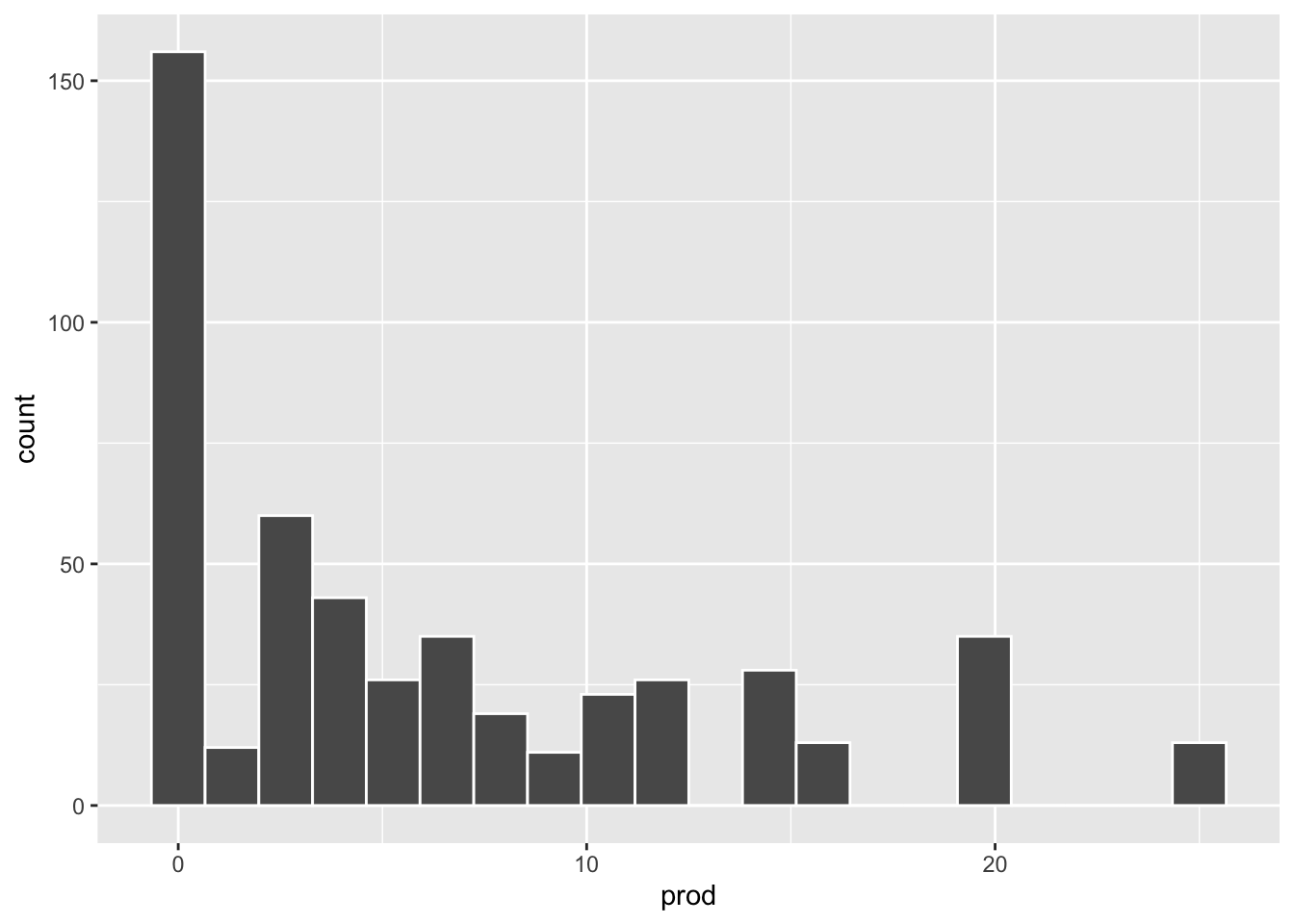

6) Sum of tickets

We have two boxes of tickets: A = [0 2 4 6] and B = [1 3 5 7]. We draw—with replacement—1 ticket from box A, and 1 ticket from box B. Let $S$ be the sum of the two tickets.

Write R code which will allow you get one simulation of this random experiment.
Write R code which will allow you to simulate 500 repetitions of this random experiment and graph the empirical distribution of $S$. Hint: the replicate() is your friend.

Show answers

R code:

box1 = c(0, 2, 4, 6)
box2 = c(1, 3, 5, 7)

sum(sample(box1, 1, replace = TRUE) + sample(box2, 1, replace = TRUE))

[1] 3

R code:

simulations = replicate(
  n = 500,
  expr = {
    sum(sample(box1, 1, replace = TRUE) + sample(box2, 1, replace = TRUE))
  }
)

data.frame(sum = simulations) |>
  ggplot(aes(x = sum)) + 
  geom_histogram(binwidth = 1, color = "white")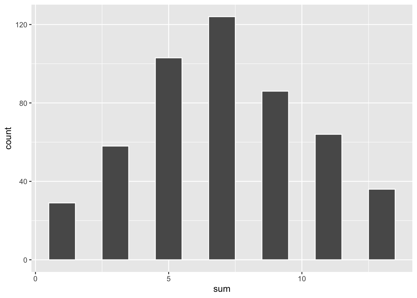

7) Great Danes

The mean gestation period for Great Danes is 70 days (expected value) with an associated variance of 2 $(\text{days})^2$. Let $Y$ be the length of pregnancy for Great Danes in terms of weeks.

What is $E(Y)$ in terms of weeks?
What is $Var(Y)$ in terms of weeks?
What is $SD(X)$ in terms of weeks?

Show answers

Let $X$ be the length of pregnancy in days, and $Y = X/7$ be the length of pregnancy in weeks. Then $E(Y) = E(X/7) = (1/7) E(X) = 70/7 = 10$ weeks
$Var(Y) = Var(X/7) = (1/49) Var(X) = 2/49 \approx 0.0408 \ \text{weeks}^2$
$SD(Y) = \sqrt{Var(Y)} = \sqrt{2/49} \approx 0.2020$ weeks

8) Two colored dice

Consider two colored 6-sided dice: one of them is a blue die, and the other is a red die. You roll the dice, and look at the numbers on their top faces. Let $V$ be a random variable that takes the following values:

\[ V = \begin{cases} 0 & \text{if both dice land on even numbers} \\ 1 & \text{if both dice land on odd numbers} \\ 2 & \text{if one die is even, and the other is odd} \end{cases} \]

Find $E(V)$
Find $Var(V)$

Show answers

First you need to find the probabilities $P(V=0) = 9/36$, $P(V=1) = 9/36$ and $P(V=2) = 18/36$.

Then find $E(V) = 0(9/36) + 1(9/36) + 2(18/36) = 1.25$
$Var(V) = E(V^2) - E(V)^2 = 0.6875$

9) Games of Chance

Consider the following games:

Game A: Consider the box [1 1 1 0 0 0]; 50 draws will be made at random with replacement from this box. On each draw, you will be paid the amount shown on the ticket, in dollars.

Game B: A die will be rolled 50 times. Each time it shows a three or a five, you win $1; on the other numbers, you win nothing.

Find the expected gain in game A
Find the expected gain in game B

Which game is better if you are betting on winning more money? Explain briefly.

Show answers

Game A

Let $X$ be the number in a single draw. $EV(X) = (0)(3/6) + (1)(3/6) = 1/2$

Let $S_X$ be the sum of the numbers in 50 draws. Notice that $S = 50X$. Thus, $EV(S_X) = 50 E(X) = 50 (1/2) = 25$

Game B

Let $Y$ be the dollar amount you win in a single roll (of a die)

\[ P(Y = y) = \begin{cases} 4/6, & \text{for } y = 0 \\ 2/6, & \text{for } y = 1 \\ \end{cases} \]

$E(Y) = (0)(4/6) + (1)(2/6) = 2/6 = 1/3$

Let $Sy$ be the total gain in 50 draws of game B, thus $EV(S_Y) = 50 E(Y) = 50 (1/3) \approx 16.66$

In summary, game A is better. In game A there are 50 draws, on each draw you have a probability of 3/6 of winning $1. In contrast, in game B there are 50 rolls, on each roll you have a probability of 2/6 of winning.