9 Data Frames
The most common format/structure for a data set is a tabular format:
with rows and columns (like a spreadsheet). When your data is in this shape,
most of the time you will work with R data frames (or similar rectangular
structures like a "matrix", "table", "tibble", etc).
Learning how to manipulate data frames is among the most important data computing skills in R. Nowadays, there are two primary approaches for manipulating data frames. One is what I call the “traditional” or “classic” approach which is what I present in this chapter. The other is the “tidy” approach which you can think of as a modern version based on the tidy data framework mainly developed by Hadley Wickham. We leave the discussion of this alternative approach for later.
To make the most of the content covered in the next sections, I am assuming that you are familiar with the rest of data objects covered in the previous chapters of part “II Data Objects in R”.
9.1 R Data Frames
A data frame is a special type of R list. In most cases, a data frame is internally stored as a list of vectors or factors, in which each vector (or factor) corresponds to a column. This implies that columns in a data frame are typically atomic structures: all elements in a given column are of the same data type. However, since a data frame is a list, you can technically have any kind of object as a column. In practice, though, having data frames with columns that are not vectors or factors is something that does not make much sense.
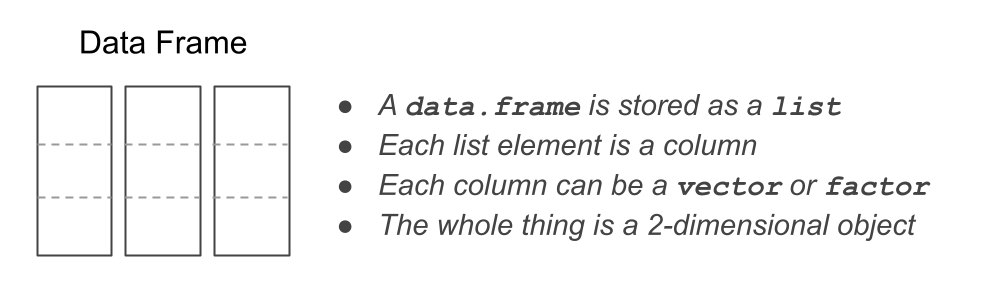
Figure 9.1: Abstract view of a data.frame
From the data manipulation point of view, data frames behave like a hybrid
object. On one hand, they are lists and can be manipulated like any other list
using double brackets dat[[ ]] and dollar operator dat$name.
On the other hand, because data frames are designed as tabular or 2-dimensional
objects, they also behave like two-dimensional arrays or matrices, admitting
bracket notation dat[ , ]. For these reasons, there is a wide array of
functions that allows you to manipulate data frames in very convenient ways.
But to the inexperienced user, all these functions may feel overwhelming.
9.2 Inspecting data frames
One of the basic tasks when working with data frames involves inspecting its contents. Specially in the early stages of data exploration, when dealing for the first time with a new data frame, you will need to inspect things like its overall structure, which includes its dimensions (number of rows and columns), the data types of its columns, the names of columns and rows, and also be able to take a peak to some of its first or last rows, and usually obtain a summary of each column.
Let’s see an example with one of the built-in data frames in R: mtcars.
Just a few rows and columns of mtcars are displayed below:
>                    mpg cyl disp  hp drat    wt
> Mazda RX4         21.0   6  160 110 3.90 2.620
> Mazda RX4 Wag     21.0   6  160 110 3.90 2.875
> Datsun 710        22.8   4  108  93 3.85 2.320
> Hornet 4 Drive    21.4   6  258 110 3.08 3.215
> Hornet Sportabout 18.7   8  360 175 3.15 3.440
The main function to explore the structure of not just a data frame, but of
any kind of object, is str(). When applied to data frames, str() returns a
report of the dimensions of the data frame, a list with the name of all the
variables, and their data types (e.g. chr character, num real, etc).
str(mtcars, vec.len = 1)
> 'data.frame': 32 obs. of  11 variables:
>  $ mpg : num  21 21 ...
>  $ cyl : num  6 6 ...
>  $ disp: num  160 160 ...
>  $ hp  : num  110 110 ...
>  $ drat: num  3.9 3.9 ...
>  $ wt  : num  2.62 ...
>  $ qsec: num  16.5 ...
>  $ vs  : num  0 0 ...
>  $ am  : num  1 1 ...
>  $ gear: num  4 4 ...
>  $ carb: num  4 4 ...
The argument vec.len = 1 is optional but we like to use it because it
indicates that just the first elements in each column should be displayed.
Observe the output returned by str(). The first line tells us that mtcars
is an object of class 'data.frame' with 32 observations (rows) and 11 variables
(columns). Then, the set of 11 variables is listed below, each line starting
with the dollar $ operator, followed by the name of the variable, followed
by a colon :, the data mode (all numeric num variables in this case),
and then a couple of values in each variable.
It is specially useful to check the data type of each column in order to catch potential issues and avoid disastrous consequences or bugs in subsequent stages.
Here’s a list of useful functions to inspect a data frame:
str(): overall structurehead(): first rowstail(): last rowssummary(): descriptive statisticsdim(): dimensionsnrow(): number of rowsncol(): number of columnsnames(): names of list elements (i.e. column names)colnames(): column namesrownames(): row namesdimnames(): list with column and row names
On a technical side, we should mention that a data frame is a list with special
attributes: an attribute names for column names, an attribute
row.names for row names, and of course its attribute class:
attributes(mtcars)
> $names
>  [1] "mpg"  "cyl"  "disp" "hp"   "drat" "wt"
>  [7] "qsec" "vs"   "am"   "gear" "carb"
>
> $row.names
>  [1] "Mazda RX4"           "Mazda RX4 Wag"
>  [3] "Datsun 710"          "Hornet 4 Drive"
>  [5] "Hornet Sportabout"   "Valiant"
>  [7] "Duster 360"          "Merc 240D"
>  [9] "Merc 230"            "Merc 280"
> [11] "Merc 280C"           "Merc 450SE"
> [13] "Merc 450SL"          "Merc 450SLC"
> [15] "Cadillac Fleetwood"  "Lincoln Continental"
> [17] "Chrysler Imperial"   "Fiat 128"
> [19] "Honda Civic"         "Toyota Corolla"
> [21] "Toyota Corona"       "Dodge Challenger"
> [23] "AMC Javelin"         "Camaro Z28"
> [25] "Pontiac Firebird"    "Fiat X1-9"
> [27] "Porsche 914-2"       "Lotus Europa"
> [29] "Ford Pantera L"      "Ferrari Dino"
> [31] "Maserati Bora"       "Volvo 142E"
>
> $class
> [1] "data.frame"
9.3 Creating data frames
Most of the (raw) data tables you will be working with will already be in some data file. However, from time to time you will face the need to create some sort of data table in R. In these situations, you will likely have to create such table with a data frame. So let’s look at various ways to “manually”” create a data frame.
Option 1: The primary option to build a data frame is with data.frame().
You pass a series of vectors (or factors), of the same length, separated by commas.
Each vector (or factor) will become a column in the generated data frame.
Preferably, give names to each column like in the example below:
dat <- data.frame(
  name = c('Anakin', 'Padme', 'Luke', 'Leia'),
  gender = c('male', 'female', 'male', 'female'),
  height = c(1.88, 1.65, 1.72, 1.50),
  weight = c(84, 45, 77, 49)
)

dat
>     name gender height weight
> 1 Anakin   male   1.88     84
> 2  Padme female   1.65     45
> 3   Luke   male   1.72     77
> 4   Leia female   1.50     49
Option 2: Another way to create data frames is with a list containing
vectors or factors (of the same length), which you then convert into a data
frame with data.frame():
# another way to create a basic data frame
lst <- list(
  name = c('Anakin', 'Padme', 'Luke', 'Leia'),
  gender = c('male', 'female', 'male', 'female'),
  height = c(1.88, 1.65, 1.72, 1.50),
  weight = c(84, 45, 77, 49)
)

tbl <- data.frame(lst)

tbl
>     name gender height weight
> 1 Anakin   male   1.88     84
> 2  Padme female   1.65     45
> 3   Luke   male   1.72     77
> 4   Leia female   1.50     49
Remember that a data.frame is nothing more than a list. So as long as the
elements in the list (vectors or factors) are of the same length, we can simply
convert the list into a data frame.
Keep in mind that in old versions of R (3.1.0 or older), data.frame() used to
convert character vectors into factors. You can always check the data type of
each column in a data frame with str():
str(tbl)
> 'data.frame': 4 obs. of  4 variables:
>  $ name  : chr  "Anakin" "Padme" "Luke" "Leia"
>  $ gender: chr  "male" "female" "male" "female"
>  $ height: num  1.88 1.65 1.72 1.5
>  $ weight: num  84 45 77 49
To prevent data.frame() from converting strings into factors, you must use
the argument stringsAsFactors = FALSE
# strings as strings (not as factors)
dat <- data.frame(
  name = c('Anakin', 'Padme', 'Luke', 'Leia'),
  gender = c('male', 'female', 'male', 'female'),
  height = c(1.88, 1.65, 1.72, 1.50),
  weight = c(84, 45, 77, 49),
  stringsAsFactors = FALSE
)

str(dat)
> 'data.frame': 4 obs. of  4 variables:
>  $ name  : chr  "Anakin" "Padme" "Luke" "Leia"
>  $ gender: chr  "male" "female" "male" "female"
>  $ height: num  1.88 1.65 1.72 1.5
>  $ weight: num  84 45 77 49
9.4 Basic Operations with Data Frames
Now that you have seen some ways to create data frames, let’s discuss a number of basic manipulations of data frames. We will show you examples of various operations, and then you’ll have the chance to put them in practice with some exercises listed at the end of the chapter.
- Selecting table elements:
- select a given cell
- select a set of cells
- select a given row
- select a set of rows
- select a given column
- select a set of columns
- Adding a new column
- Deleting a column
- Renaming a column
- Moving a column
- Transforming a column
Let’s say you have a data frame dat with the following content:
dat <- data.frame(
  name = c('Leia', 'Luke', 'Han'),
  gender = c('female', 'male', 'male'),
  height = c(1.50, 1.72, 1.80),
  jedi = c(FALSE, TRUE, FALSE),
  stringsAsFactors = FALSE
)

dat
  name gender height  jedi
1 Leia female   1.50 FALSE
2 Luke   male   1.72  TRUE
3  Han   male   1.80 FALSE
9.4.1 Selecting elements
The data frame dat is a 2-dimensional object: the 1st dimension corresponds
to the rows, while the 2nd dimension corresponds to the columns.
Because dat has two dimensions, the bracket notation involves
working with data frames in this form: dat[ , ].
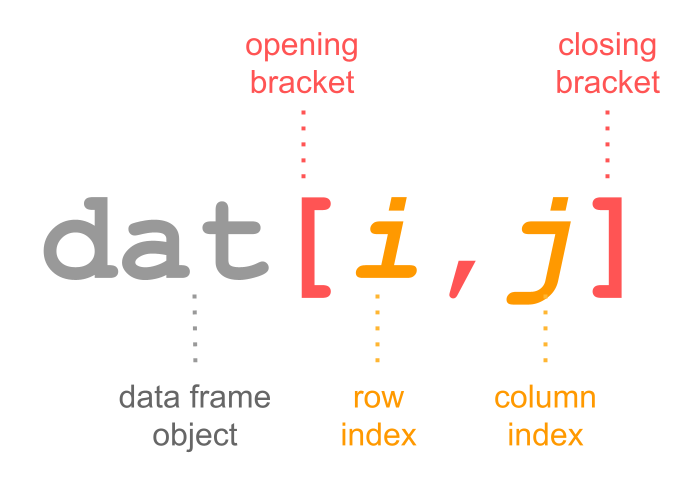
Figure 9.2: Bracket notation in data frames
In other words, you have to specify values inside the
brackets for the 1st index, and the 2nd index: dat[index1, index2].
Selecting cells
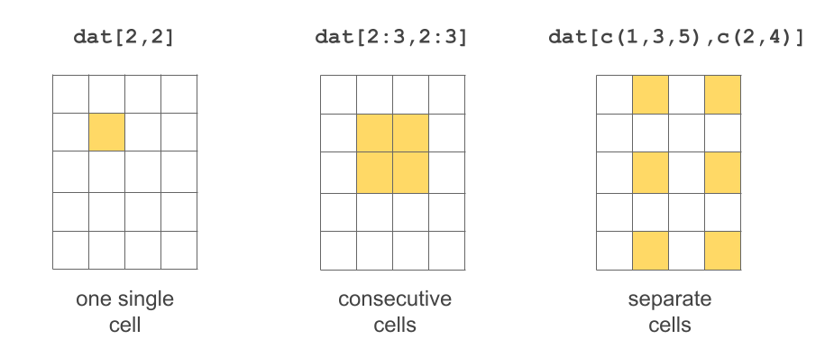
Figure 9.3: Several ways to select cells
# select value in row 1 and column 1
dat[1,1]
> [1] "Leia"

# select value in row 2 and column 3
dat[2,3]
> [1] 1.72

# select values in these cells
dat[1:2,3:4]
>   height  jedi
> 1   1.50 FALSE
> 2   1.72  TRUE
It is also possible to exclude certain rows-and-columns by passing negative numeric indices:
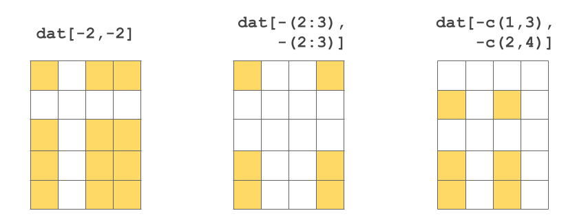
Figure 9.4: Several ways to exclude cells
Selecting rows
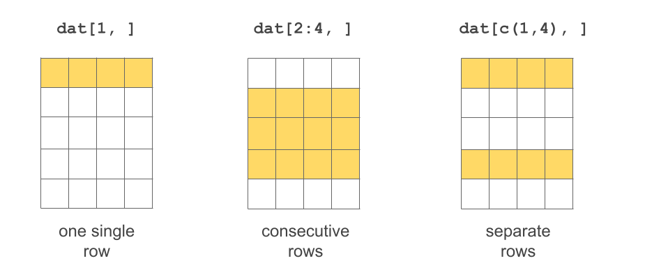
Figure 9.5: Several ways to select rows
If no value is specified for index1 then all rows are included. Likewise,
if no value is specified for index2 then all columns are included.
# selecting first row
dat[1, ]
>   name gender height  jedi
> 1 Leia female    1.5 FALSE

# selecting third row
dat[3, ]
>   name gender height  jedi
> 3  Han   male    1.8 FALSE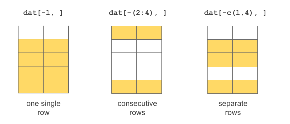
Figure 9.6: Several ways to exclude rows
Selecting columns
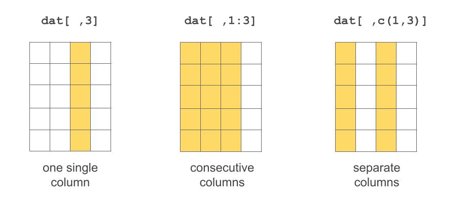
Figure 9.7: Several ways to select columns
# selecting second column
dat[ ,2]
> [1] "female" "male"   "male"

# selecting columns 2 to 4
dat[ ,2:4]
>   gender height  jedi
> 1 female   1.50 FALSE
> 2   male   1.72  TRUE
> 3   male   1.80 FALSE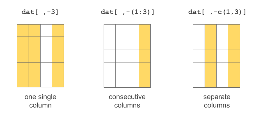
Figure 9.8: Several ways to exclude columns
More Options to Access Columns
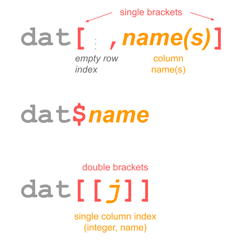
Figure 9.9: Other options to select columns of a data frame
The dollar sign also works for selecting a column of a data frame using its name
mtcars$mpg
>  [1] 21.0 21.0 22.8 21.4 18.7 18.1 14.3 24.4 22.8
> [10] 19.2 17.8 16.4 17.3 15.2 10.4 10.4 14.7 32.4
> [19] 30.4 33.9 21.5 15.5 15.2 13.3 19.2 27.3 26.0
> [28] 30.4 15.8 19.7 15.0 21.4
You don’t need to use quote marks, but you can if you want. The following calls are equivalent.
mtcars$'mpg'
mtcars$"mpg"
mtcars$`mpg`
9.4.2 Adding a column
Perhaps the simplest way to add a column is with the dollar operator $.
You just need to give a name for the new column, and assign a vector (or factor):
# adding a column
dat$new_column <- c('a', 'e', 'i')
dat
>   name gender height  jedi new_column
> 1 Leia female   1.50 FALSE          a
> 2 Luke   male   1.72  TRUE          e
> 3  Han   male   1.80 FALSE          i
Another way to add a column is with the column binding function cbind():
# vector of weights
weight <- c(49, 77, 85)

# adding weights to dat
dat <- cbind(dat, weight)
dat
>   name gender height  jedi new_column weight
> 1 Leia female   1.50 FALSE          a     49
> 2 Luke   male   1.72  TRUE          e     77
> 3  Han   male   1.80 FALSE          i     85
9.4.3 Deleting a column
The inverse operation of adding a column consists of deleting a column.
This is possible with the $ dollar operator. For instance, say you want to
remove the column new_column. Use the $ operator to select this column,
and assign it the value NULL (think of this as NULLifying a column):
# deleting a column
dat$new_column <- NULL
dat
>   name gender height  jedi weight
> 1 Leia female   1.50 FALSE     49
> 2 Luke   male   1.72  TRUE     77
> 3  Han   male   1.80 FALSE     85
9.4.4 Renaming a column
What if you want to rename a column? There are various options to do this.
One way is by changing the column names attribute:
# attributes
attributes(dat)
> $names
> [1] "name"   "gender" "height" "jedi"   "weight"
>
> $row.names
> [1] 1 2 3
>
> $class
> [1] "data.frame"
which is more commonly accessed with the names() function:
# column names
names(dat)
> [1] "name"   "gender" "height" "jedi"   "weight"
Notice that dat has a list of attributes. The element names is the vector
of column names.
You can directly modify the vector of names; for example let’s change
gender to sex:
# changing rookie to rooky
attributes(dat)$names[2] <- "sex"

# display column names
names(dat)
> [1] "name"   "sex"    "height" "jedi"   "weight"
By the way: this approach of changing the name of a variable is very low level, and probably unfamiliar to most useRs.
9.4.5 Moving a column
A more challenging operation is when you want to move a column to a different
position. What if you want to move salary to the last position (last column)?
One option is to create a vector of column names in the desired order, and then
use this vector (for the index of columns) to reassign the data frame like this:
reordered_names <- c("name", "jedi", "height", "weight", "sex")
dat <- dat[ ,reordered_names]
dat
>   name  jedi height weight    sex
> 1 Leia FALSE   1.50     49 female
> 2 Luke  TRUE   1.72     77   male
> 3  Han FALSE   1.80     85   male
9.4.6 Transforming a column
A more common operation than deleting or moving a column, is to transform the
values in a column. This can be easily accomplished with the $ operator.
For instance, let’s say that we want to transform height from meters to
centimeters:
# converting height to centimeters
dat$height <- dat$height * 100
dat
>   name  jedi height weight    sex
> 1 Leia FALSE    150     49 female
> 2 Luke  TRUE    172     77   male
> 3  Han FALSE    180     85   male
Likewise, instead of using the $ operator, you can refer to the column using
bracket notation. Here’s how to transform weight from kilograms to pounds
(1 kg = 2.20462 pounds):
# weight into pounds
dat[ ,"weight"] <- dat[ ,"weight"] * 2.20462
dat
>   name  jedi height   weight    sex
> 1 Leia FALSE    150 108.0264 female
> 2 Luke  TRUE    172 169.7557   male
> 3  Han FALSE    180 187.3927   male
There is also the transform() function which transform values interactively,
that is, temporarily:
# transform weight to kgs
transform(dat, weight = weight / 0.453592)
>   name  jedi height   weight    sex
> 1 Leia FALSE    150 238.1576 female
> 2 Luke  TRUE    172 374.2476   male
> 3  Han FALSE    180 413.1305   male
transform() does its job of modifying the values of weight but only
temporarily; if you inspect dat you’ll see what this means:
# did weight really change?
dat
>   name  jedi height   weight    sex
> 1 Leia FALSE    150 108.0264 female
> 2 Luke  TRUE    172 169.7557   male
> 3  Han FALSE    180 187.3927   male
To make the changes permanent with transform(), you need to reassign them
to the data frame:
# transform weight to inches (permanently)
dat <- transform(dat, weight = weight / 0.453592)
dat
>   name  jedi height   weight    sex
> 1 Leia FALSE    150 238.1576 female
> 2 Luke  TRUE    172 374.2476   male
> 3  Han FALSE    180 413.1305   male
9.5 Exercises
1) Consider the following data frame df:
      first      last  gender  born         spell
1     Harry    Potter    male  1980  sectumsempra
2  Hermione   Granger  female  1979     alohomora
3       Ron   Weasley    male  1980    riddikulus
4      Luna  Lovegood  female  1981       episkey
What commands will fail to return the data of individuals born in 1980?
df[c(TRUE, FALSE, TRUE, FALSE), ]df[df[,4] == 1980, ]df[df$born == 1980]df[df$born == 1980, ]df[ ,df$born == 1980]
Select the command that does not provide information about the data frame
df:head(df)str(df)tail(df)rm(df)summary(df)
Your friend is trying to display the first three rows on columns 1 (
first) and 2 (last), by unsuccessfully using the following command. Why does the command print all columns?
df[1:3, 1 & 2]
>      first    last gender born        spell
> 1    Harry  Potter   male 1980 sectumsempra
> 2 Hermione Granger female 1979    alohomora
> 3      Ron Weasley   male 1980   riddikulus
Write a command that would correctly display the first two columns.
Write a command that would give you the following data from
df.
         spell    first
1 sectumsempra    Harry
2    alohomora Hermione
3   riddikulus      Ron
4      episkey     Luna
2) Consider the following data frame dat
       first        last   gender      title
1        Jon        Snow     male       lord
2       Arya       Stark   female   princess
3     Tyrion   Lannister     male     master
4   Daenerys   Targaryen   female   khaleesi
5       Yara     Greyjoy   female   princess
    gpa
1   2.8
2   3.5
3   2.9
4   3.7
5    NA
One of your friends wrote the following R code. Help your friend find all the errors and explain what’s wrong.
# value of 'first' associated to maximum 'gpa'
max_gpa <- max(dat$gpa, na.rm = TRUE)
which_max_gpa <- dat$gpa = max_gpa
dat$first(which_max_gpa)

# gpa of title lord
dat$gpa[dat[ ,title] = "lord"]

# median gpa (of each gender)
which_males <- dat$gender == 'male'
which_females <- dat$gender == 'female'
median_females <- median(dat$gpa[which_males])
median_males <- median(dat$gpa[which_males])