11 More Base Graphics
R comes with many functions that let us produce a wide variety of graphics, plots, diagrams, charts, maps, … you name it.
In this chapter we describe the behavior of the plot() method and it
can be used to produce a large number of graphics.
11.1 The plot() function
plot() is the most important high-level function in traditional graphics
The first argument to
plot()provides the data to plotThe provided data can take different forms: e.g. vectors, factors, matrices, data frames.
To be more precise,
plot()is a generic functionYou can create your own
plot()method function
In its basic form, we can use plot() to make graphics of:
one single variable
two variables
multiple variables
11.2 One variable graphics
High-level graphics of a single variable
| Function | Data | Graphic |
|---|---|---|
plot() |
numeric | scatterplot |
plot() |
factor | barplot |
plot() |
1-D table | barplot |
A numeric object can be either a vector or a 1-D array (e.g. row or column
from a matrix)
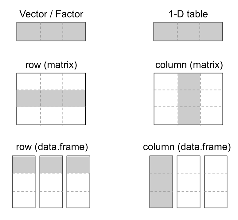
Figure 11.1: One-variable objects can take multiple forms.
Here’s an example:
# plot numeric vector
num_vec <- (c(1:10))^2
plot(num_vec)

# plot factor
set.seed(4)
abc <- factor(sample(c('A', 'B', 'C'), 20, replace = TRUE))
plot(abc)

# plot 1D-table
abc_table <- table(abc)
plot(abc_table)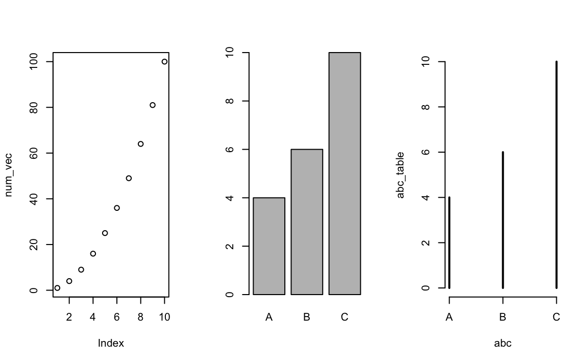
11.2.1 More high-level graphics of a single variable
| Function | Data | Graphic |
|---|---|---|
barplot() |
numeric | barchart |
pie() |
numeric | piechart |
dotchart() |
numeric | dotplot |
boxplot() |
numeric | boxplot |
hist() |
numeric | histogram |
stripchart() |
numeric | 1-D scatterplot |
stem() |
numeric | stem-and-leaf plot |
Examples: one signle variable plots
# barplot numeric vector
barplot(num_vec)

# pie chart
pie(1:3)

# dot plot
dotchart(num_vec)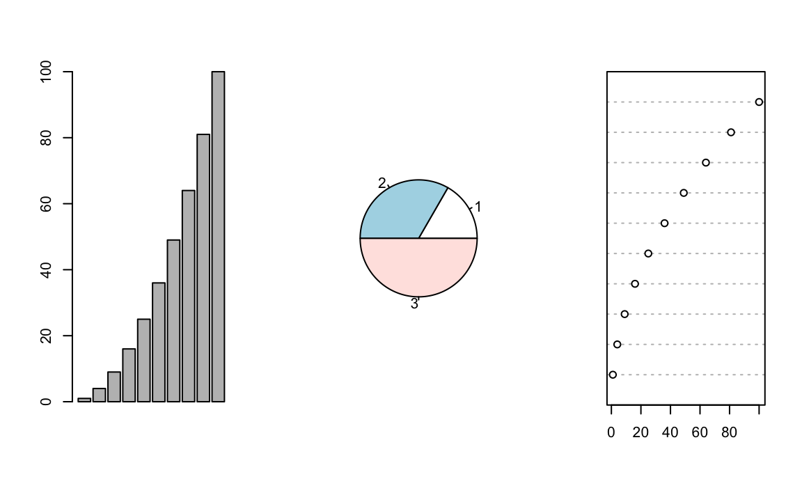
Examples: one single variable plots
# barplot numeric vector
boxplot(num_vec)

# pie chart
hist(num_vec)

# dot plot
stripchart(num_vec)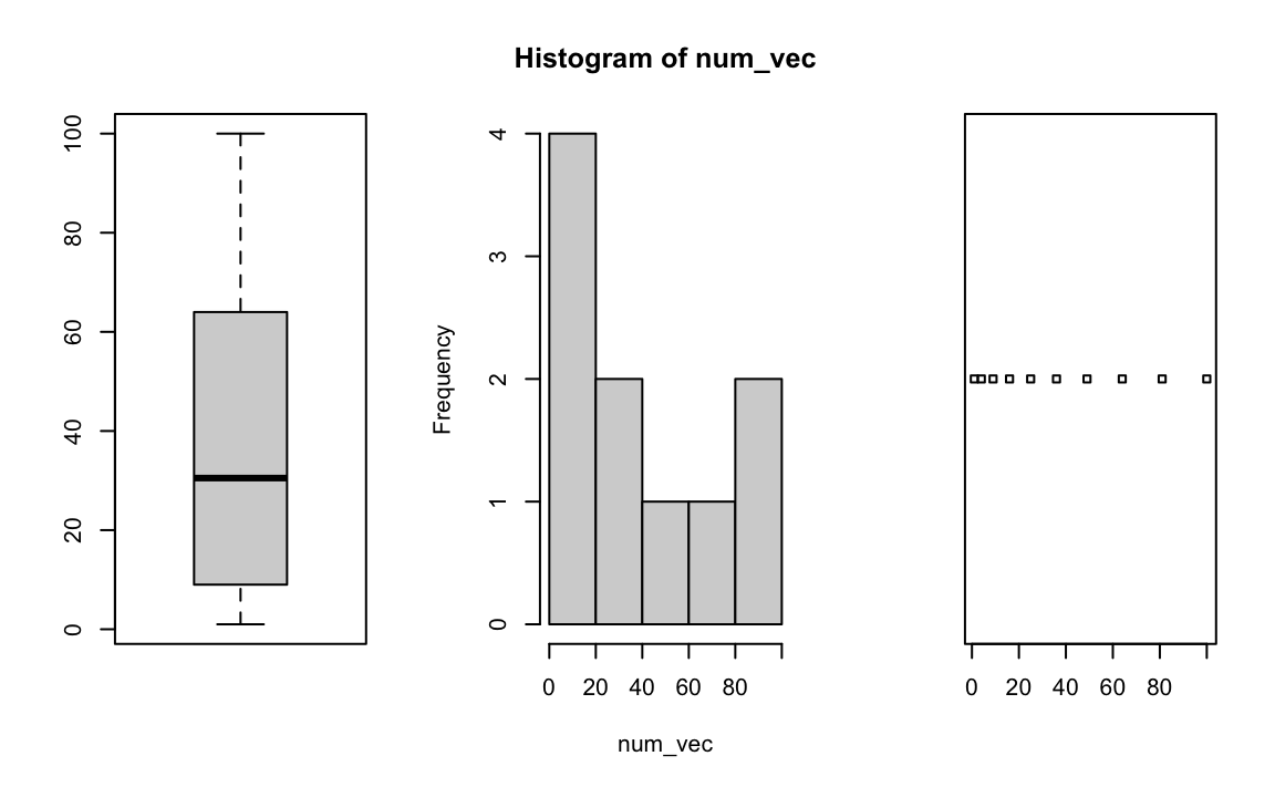
11.3 Plots of Two Variables
| Function | Data | Graphic |
|---|---|---|
plot() |
numeric | scatterplot |
plot() |
numeric | stripcharts |
plot() |
factor | boxplots |
plot() |
factor | spineplot |
plot() |
2-column numeric matrix | scatterplot |
plot() |
2-column numeric data.frame | scatterplot |
plot() |
2-D table | mosaicplot |
A numeric object can be either a vector or a 1-D array (e.g. row or column
from a matrix)
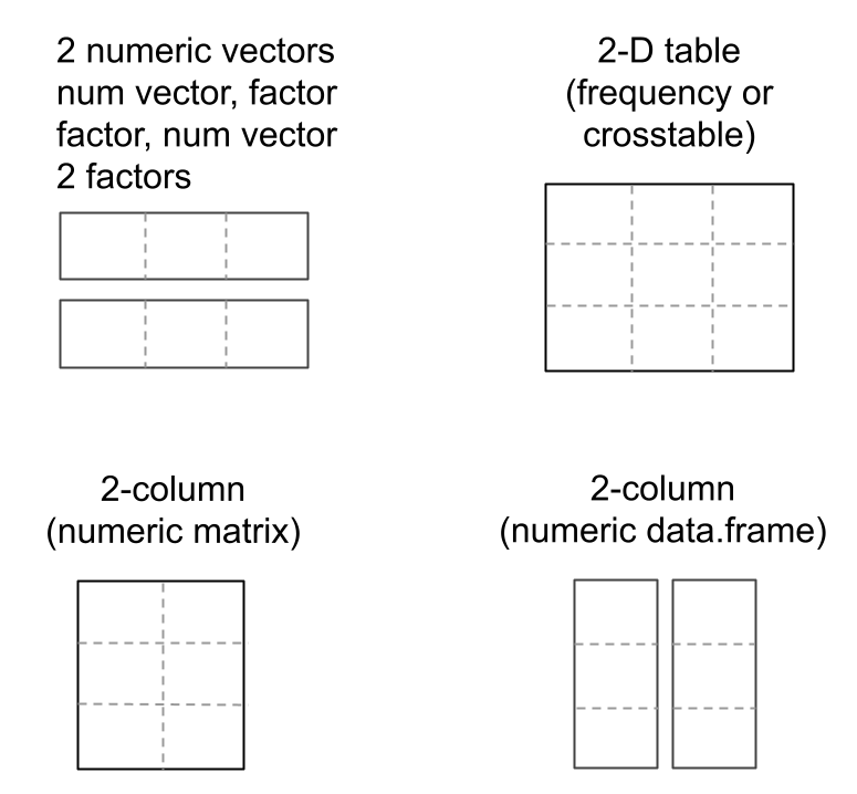
Figure 11.2: One-variable objects can take multiple forms.
Here’s an example:
# plot numeric, numeric
plot(iris$Petal.Length, iris$Sepal.Length)
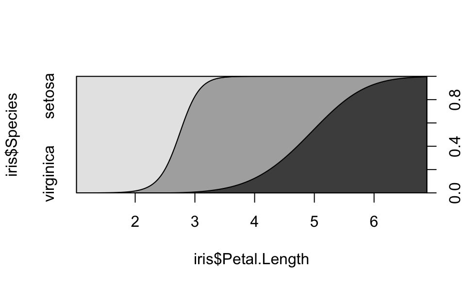
# plot numeric, factor
plot(iris$Petal.Length, iris$Species)
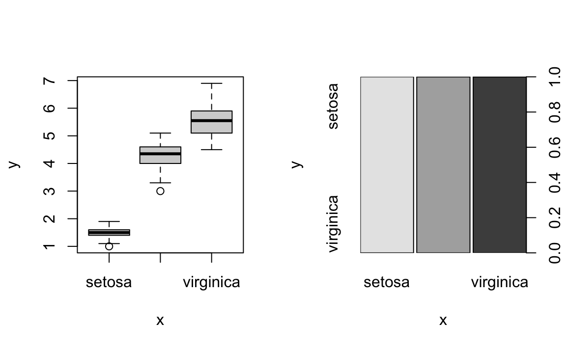
# plot factor, numeric
plot(iris$Species, iris$Petal.Length)
# plot factor, factor
plot(iris$Species, iris$Species)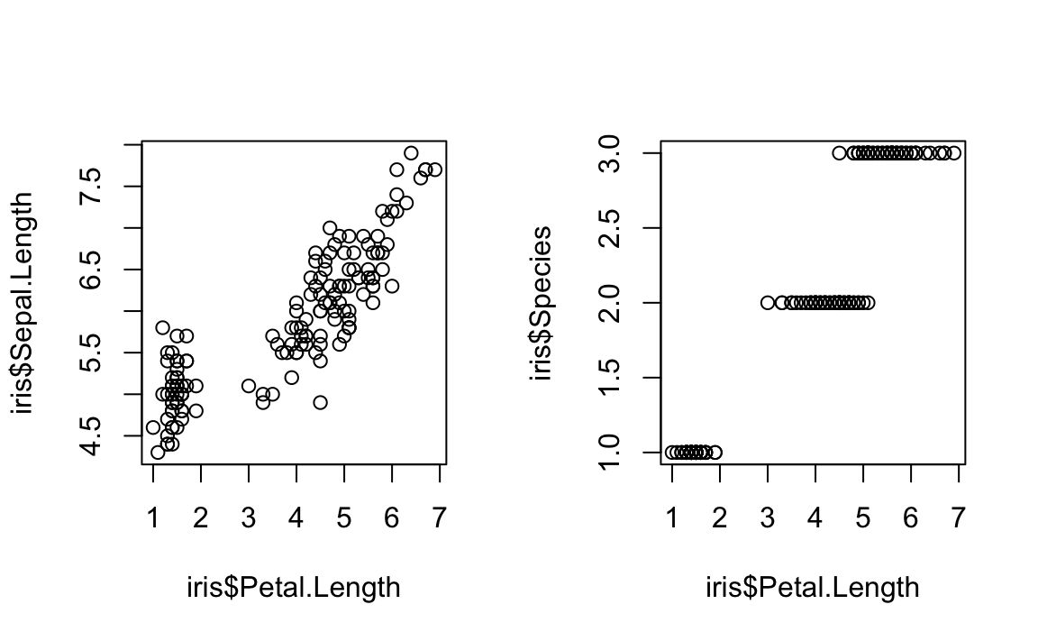
11.3.1 Example: Plots of two variables
# some fake data
set.seed(1)

# hair color
hair <- factor(
  sample(c('blond', 'black', 'brown'), 100, replace = TRUE))

# eye color
eye <- factor(
  sample(c('blue', 'brown', 'green'), 100, replace = TRUE))
# plot factor, factor
plot(hair, eye)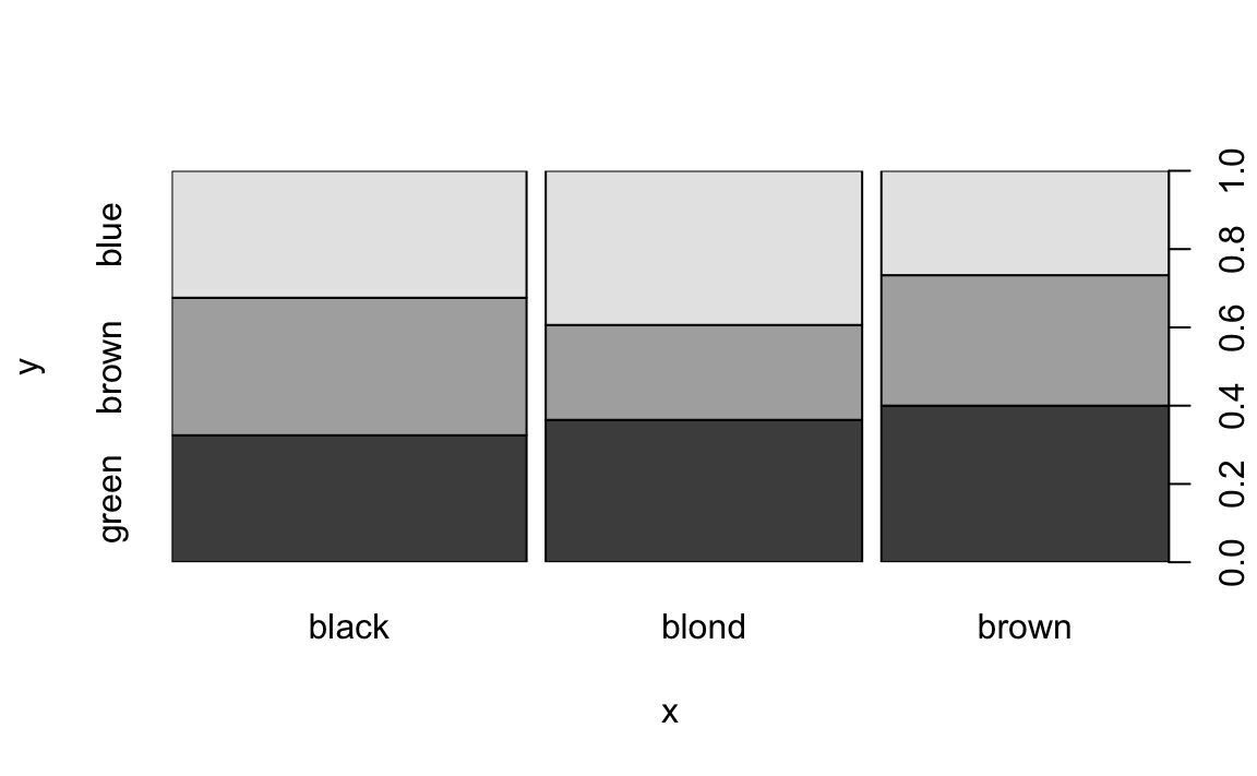
11.3.2 More high-level graphics of two variables
| Function | Data | Graphic |
|---|---|---|
sunflowerplot() |
numeric, numeric | sunflower scatterplot |
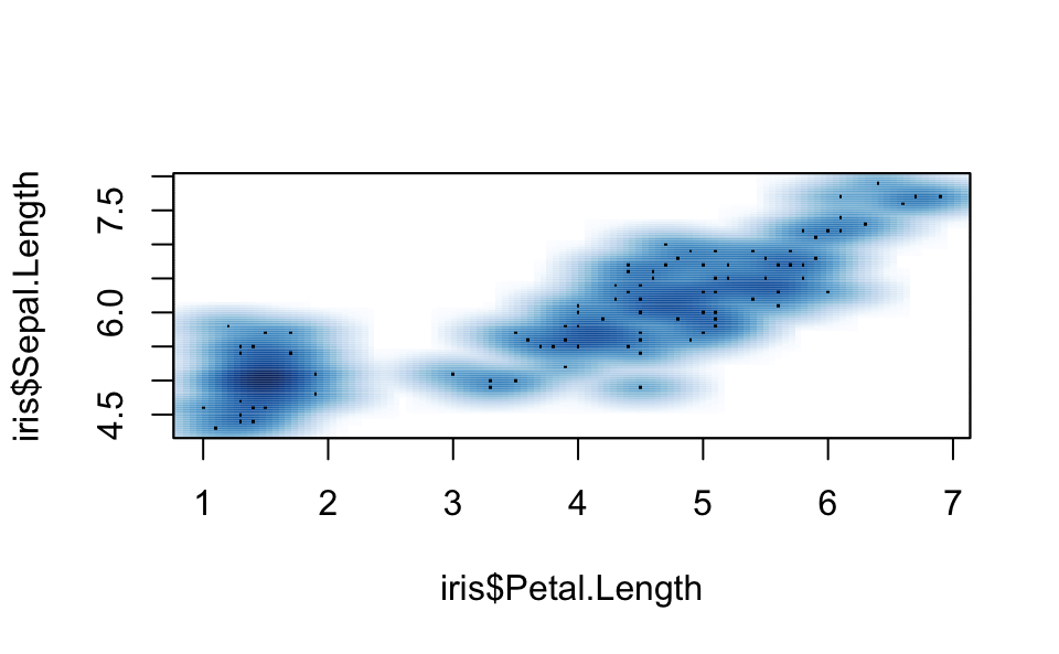
smoothScatter() |
numeric, numeric | smooth scatterplot |
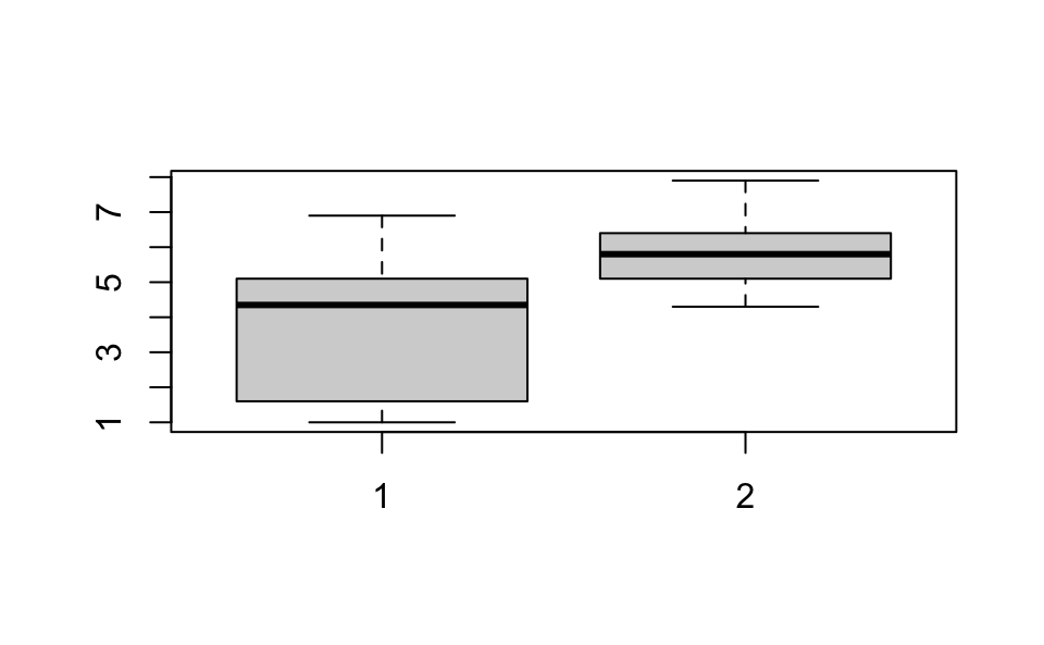
boxplot() |
list of numeric | boxplots |
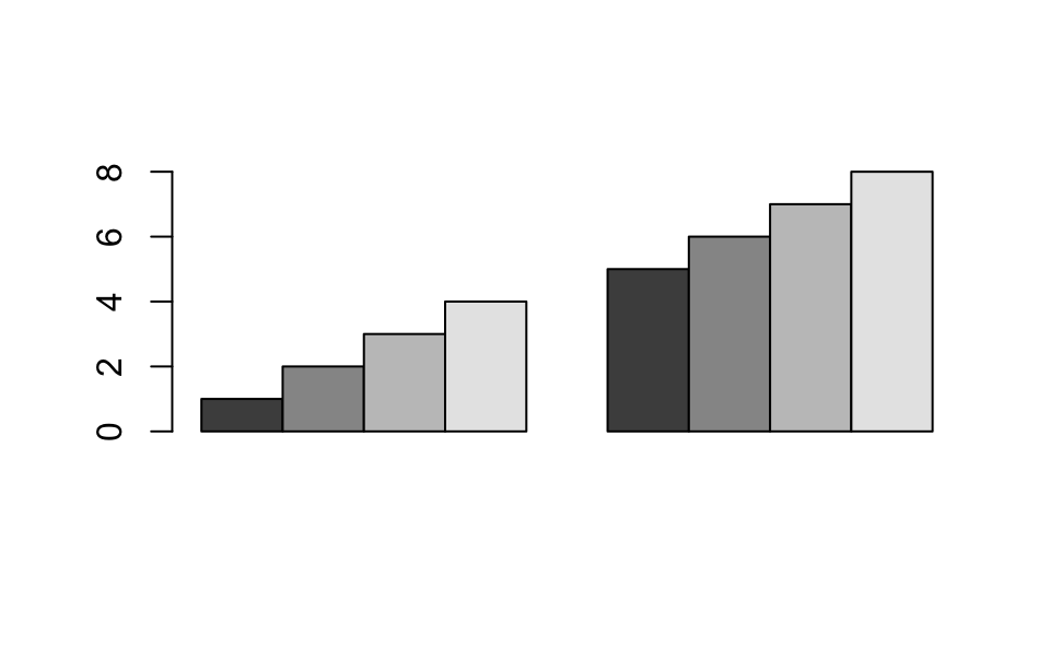
barplot() |
matrix | stacked barplot |
dotchart() |
matrix | dotplot |
stripchart() |
list of numeric | stripcharts |
spineplot() |
numeric, factor | spinogram |
cdplot() |
numeric, factor | conditional density plot |
fourfoldplot() |
2x2 table | fourfold display |
assocplot() |
2-D table | association plot |
mosaicplot() |
2-D table | mosaicplot |
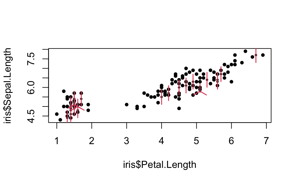
Sunflower plot
# sunflower plot (numeric, numeric)
sunflowerplot(iris$Petal.Length, iris$Sepal.Length)