31 De Mere’s Games
In this chapter, we will put in practice the concepts that we’ve covered so far about data objects and programming structures, applied to simulation and probability problems.
31.1 Probability Example
We are going to use a classic example in the history of probability: the problem posed by French gambler Antoine Gombaud, better known by his nome de plume “Chevalier De Méré”. He was not a nobleman, but just an amateur mathematician, and avid gambler.
We are studying two games: game 1 and game 2
31.1.1 Game 1
In version 1, you roll a die four times, and you win if you get at least one six.

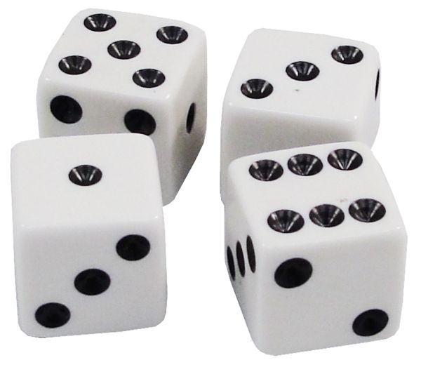
Figure 31.1: Game version 1: roll a pair of dice
What could happen when rolling one die four times? Some possible outcomes:
1, 3, 5, 2(you lose)2, 4, 6, 5(you win)5, 6, 3, 6(you win)
This is how De Méré was reasoning about game 1:
- the chance of getting a six in one roll of a die is 1/6 (this is correct)
- in four rolls of a die, the chance of getting one six would be \(4 \times 1/6 = 4/6 = 2/3\) (this is incorrect)
31.1.2 Game 2
Despite De Méré’s faulty reasoning about the probability of getting one six in four rolls, he was able to make money by playing version 1 of the game. He also wanted to make things more interesting and he deviced a second version of the game. Instead of rolling one die, he decided to roll a pair of dice. The outcome of interest was going to be getting a double six. And the tricky part was deciding how many times to roll the dice.
He correctly guessed that the chance of getting one double six when you roll a pair of dice is 1/36. What he incorrectly calculated was the probability of winning in this version 2. The problem had to do with his faulty reasoning from the second assumption in game 1.
He wanted to keep the same (faulty) proportion in game-1 of \(4/6 = 2/3\) to game-2. To keep this proportion, he calculated that the number of rolls—of a pair of dice—had to be 24 times.
\[ \frac{4}{6} = \frac{x}{36} \quad \longrightarrow \quad x = 24 \]
He incorrectly calculated that in 24 rolls of a pair of dice, the chance of getting one double six would be 24/36 = 2/3.
So in version 2, a player rolls a pair of dice 24 times, and they win if they get at least one double-six.
Unfortunately, with game 2 De Méré was losing money, and he did not understand why. He turned into Blaise Pascal for some help, who in turn contacted Pierre de Fermat exchanging correspondence in the 1650s.
Here’s an extract from a letter written by Pascal to Fermat, posing the problem that De Méré was facing:
If one undertakes to throw a six with one die, the advatange of undertaking it in 4 throws is as 671 to 625. If one undertakes to throw a double-six with two dice, there is a disadvantage of undertaking it in 24 throws. And nevertheless 24 is to 36 (which is the number of faces of two dice) as 4 to 6 (which is the number of faces of one die).
31.1.3 Binomial Probability
The answer to De Méré’s question can be easily calculated with binomial probability formulas. Let’s do the math.
Probability of winning in game 1
In game 1, we know that the probability of getting no six in a single roll is:
\[ P(\text{no six in one roll}) = \frac{5}{6} \]
In turn, the probability of no six in four rolls involves not getting a six in the first roll, AND not getting a six in the second roll, AND not getting a six in the third roll, AND not getting a six in the fourth roll:
\[\begin{align*} P(\text{no six in 4 rolls}) &= P(\text{no six in roll 1}) \times \dots \times P(\text{no six in roll 4}) \\ &= \frac{5}{6} \times \frac{5}{6} \times \frac{5}{6} \times \frac{5}{6} \\ &= \left( \frac{5}{6} \right)^4 \\ &= \frac{625}{1296} = 0.482253 \end{align*}\]
Consequently, the probability of winning a game is:
\[ P(\text{at least one six in 4 rolls}) = 1 - \left( \frac{5}{6} \right)^4 = 0.517747 \]
Note that this probability is not that different from 0.5, just slightly greater than 0.5. But the difference is enough so that if you gamble in this game, you should expect to have a positive gain … in the long run.
Probability of winning in game 2
In game 2, we know that the probability of getting no double six when rolling a pair of dice is:
\[ P(\text{no double six when rolloing a pair of dice}) = \frac{35}{36} \]
In turn, the probability of no double six when rolling a pair of dice 24 times is:
\[ P(\text{no double six in 24 rolls}) = \left(\frac{35}{36}\right)^{24} = 0.5086 \]
Consequently, the probability of winning a game is:
\[ P(\text{at least one double six in 24 rolls}) = 1 - 0.5086 = 0.4914 \]
Note also that in this case, this probability is not that different from 0.5, just slightly less than 0.5. But the difference is enough so that if you gamble in this game, you should expect to have a negative gain (i.e. loss) … in the long run.
Simulations Perspective
Rather than solving the problem analytically, we can simulate 4 rolls of a die and count the number of 6’s. If we simulate rolling 4 dice many times, then the proportion of times we get 0, 1, 2, 3, or 4 sixes should be close to the chance of that many sixes on any 4 rolls.
Some Questions:
- What is the chance of getting one 6 when rolling a die?
- What is the chance of getting one 6 when rolling two dice?
- What is the chance of getting at least one 6 when rolling 4 dice?
What are the steps?
- Simulate rolling one die
- Simulate rolling a pair of dice
- Simulate rolling four dice
- Count the number of sixes
31.1.4 Simulating one die
Let’s start by simulating one die.

Figure 31.2: Simulating one die
This can easily be done with a numeric sequence vector to create a die object:
Then comes rolling the die, using sample()
set.seed(5)
sample(die, size = 1)
#> [1] 2
sample(die, size = 1)
#> [1] 3
sample(die, size = 1)
#> [1] 1
To make things more convenient, it’s better if we write a rolldie() function.
Here’s one option for this function—and you may come up with other alternatives.
31.1.5 Rolling a pair of dice
Because in game 2 we need to roll a pair of dice, we could also write another
auxiliary function roll2(). Here’s some code for such a function:
# pair of dice function
roll2 <- function() {
  die <- 1:6
  rol1 <- sample(die, size = 1)
  rol2 <- sample(die, size = 1)
  c(rol1, rol2)
}
After inspecting the code, we hope that you can identify some unnecessary repetition:
# pair of dice function
roll2 <- function() {
  die <- 1:6
  rol1 <- sample(die, size = 1)
  rol2 <- sample(die, size = 1)  # repeated command!
  c(rol1, rol2)
}
Instead of calling smaple() twixe, we can just call it one, and use its
argument size = 2 to indicate two rolls:
Now try it:
for (i in 1:15) {
  print(sample(die, size = 2))
}
#> [1] 5 3
#> [1] 3 2
#> [1] 5 4
#> [1] 2 5
#> [1] 3 1
#> [1] 6 4
#> [1] 3 2
#> [1] 5 2
#> [1] 2 3
#> [1] 1 2
#> [1] 6 4
#> [1] 5 3
#> [1] 6 2
#> [1] 1 2
#> [1] 2 4

# Can you spot a problem?
The problem is that none of the above samples have repeated numbers. For
instance, there is no 1 1, or 2 2, or 6 6. Why? Becasue the function
sample() draws random samples without replacement by default.
Instead, we need to sample with replacement. This is done with the argument
replace = TRUE:
Let’s create a more general function to roll a die any number of times
Now we can roll several dice:
31.1.6 De Mere’s Game 1
Now that we have our roll() function that allows to roll a die any number
of times, let’s write some code generate 100 simulations of repetitions of
game-1. To store the outputs in each simulation, we can use a matrix with
four columns and 100 rows. In eaah row, we store the vector of numbers from
rolling a die four times.
set.seed(2)
# play 100 times
results <- matrix(0, nrow = 100, ncol = 4)

for (i in 1:100) {
  results[i, ] <- roll(times = 4)
}

head(results)
#>      [,1] [,2] [,3] [,4]
#> [1,]    5    6    6    1
#> [2,]    5    1    4    5
#> [3,]    1    2    3    1
#> [4,]    3    6    2    3
#> [5,]    1    6    1    4
#> [6,]    3    6    1    6
With the matrix results, we can see which simulations (which games) have
at least one six. For example, the first game—first row—has 2 sixes, which
meets the winning condition of “at least one six”
In contrast, the second game—second row—has no sixes, which represents losing this game:
Let’s compute proportion of wins:
counts <- 0

for (i in 1:100) {
  if (any(results[i, ] == 6))
    counts <- counts + 1
}

# proportion of wins
counts / 100
#> [1] 0.55
For illustration purposes, instead of using a for loop, let’s see how to
accomplish the same computation with the apply() function. Recall that this
function takes an array and applies a function to all the elements in the
specified MARGIN (MARGIN = 1 for rows, MARGIN = 2 for columns).
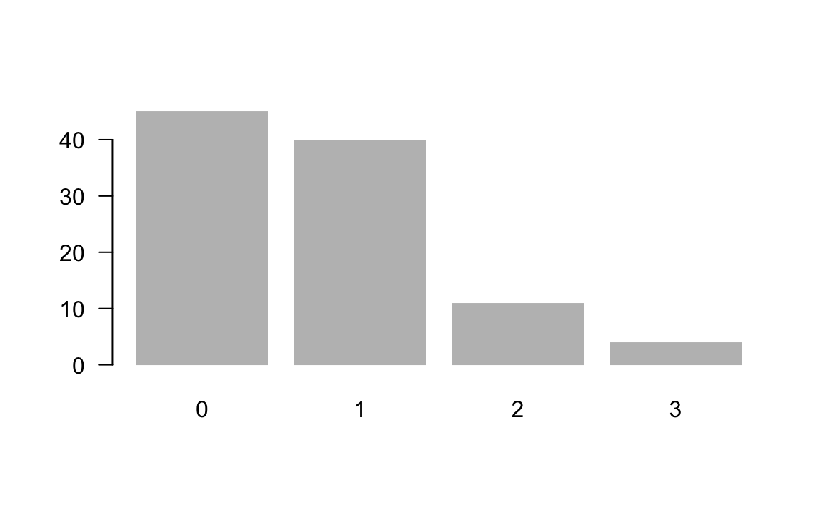
sixes <- apply(results, MARGIN = 1, function(x) sum(x == 6))

table(sixes)
#> sixes
#>  0  1  2  3
#> 45 40 11  4

# rolls with at least one six
sum(table(sixes)[-1])
#> [1] 55
Finally, we can graph the frequencies for the possible number of sixes out of the 100 simulations:

Considerations
- How would you make the code more flexible?
- What type of parameters?
- How would you avoid repetition?
31.1.7 De Mere’s Game 2
We know that the second version of the game involves:
- Two dice
- 24 rolls
- Win: getting at least one double 6
# function to roll a pair of dice, a given number of times
roll2 <- function(times = 1) {
  dice2 <- unlist(lapply(1:6, function(x) x + 1:6))
  sample(dice2, size = times, replace = TRUE)
}

roll2()
#> [1] 9
roll2(24)
#> [1] 2 5 10 6 8 7 2 8 8 4 4 9 10 7 7 8 8 6 4 10 3 5 5 4- It’s better if we sum the points of rolling two dice
- Possible outcomes: \(\{2, 3, 4, \dots, 10, 11, 12\}\)
- Double six is equivalent to 12 points
set.seed(139)
games <- 10000
results <- matrix(0, nrow = games, ncol = 24)

for (i in 1:games) {
  results[i, ] <- roll2(24)
}

doublesix <- apply(results, 1, function(x) sum(x == 12))
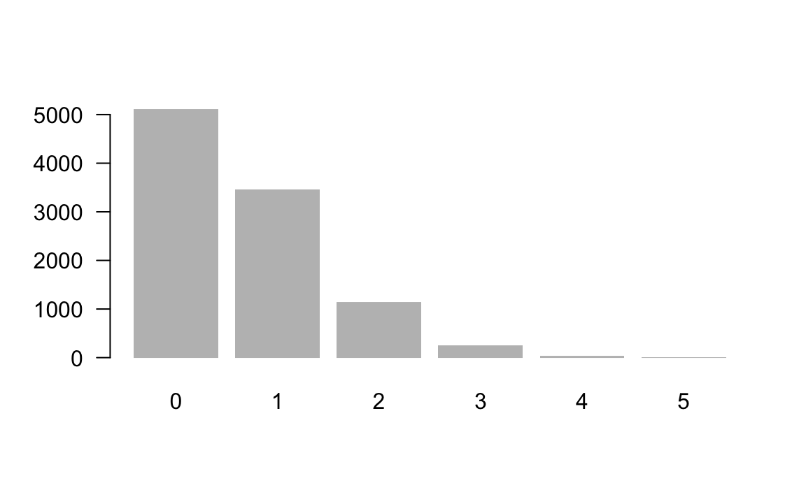
table(doublesix)
#> doublesix
#>    0    1    2    3    4    5
#> 5107 3460 1140  247   42    4

sum(table(doublesix)[-1])
#> [1] 4893
Let’s graph the obtained results:

and get estimated proportions: