18 Introduction

This part of the book is entirely dedicated to “all things tables”. We aim to provide a comprehensive review of the fundamental concepts related to tables. Some of the concepts are language agnostic concepts that are universal to every data analysis project (e.g. common formats of storing tabular data, good practices to handle data tables, tidyness). Other concepts are more specific to how R handles rectangular data. Likewise, there are also other manipulations that can be done outside R, with the use of what we call data technologies (in part VII of the book).

Most of the material in this chapter is borrowed from Gaston Sanchez’s book A Matrix Algebra Companion for Statistical Learning (with permission from the author).

18.1 Data: Individuals and Variables

To illustrate some of the ideas presented in this chapter we’re going to use a toy example with data of three individuals from a galaxy far, far away: Leia Organa, Luke Skywalker, and Han Solo.

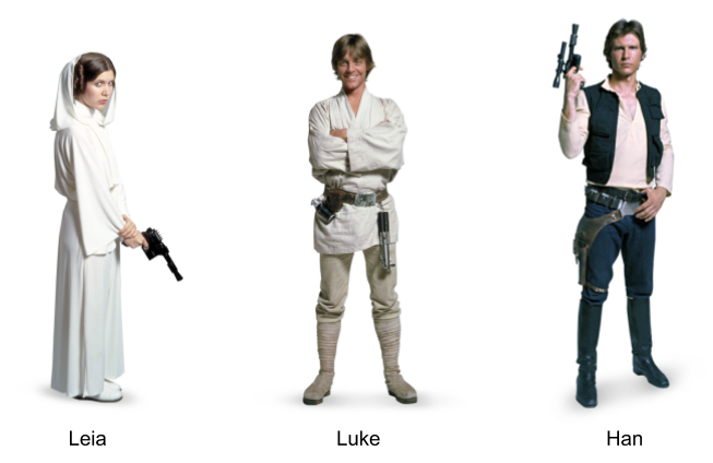
Figure 18.1: Three individuals

In particular, let’s consider the following information about these subjects:

• Leia is a woman, 150 centimeters tall, and weighs 49 kilograms.

• Luke is a man, 172 centimeters tall, and weighs 77 kilograms.

• Han is a man, 180 centimeters tall, and weighs 80 kilograms.

We can say that the above information lists characteristics of three individuals. Or put in an equivalent way, that three subjects are described based on some of their characteristics: Name, Sex, Height, and Weight. Using statistical terminology, we formally say that we have data consisting of three individuals described by some variables.

Statistical terminology is abundant and you’ll find that individuals are also known as observations, cases, objects, samples or items. Example of individuals can be people, animals, plants, planets, spaceships, countries, or any other kind of object.

A variable is any characteristic of an individual. Sometimes we refer to variables as features, aspects, indicators, descriptors, or properties that we measure or observe on individuals.

This combo of individuals and variables is perhaps the most common conceptualization of the term “data” within statistics. Within computer science communities, the common convention is to refer to the same type of combo as cases and features. However, bear in mind that there are other ways in which analysts and researchers think about data.

18.1.1 Representing Data

Assuming that our sample data consists of Name, Sex, Height and Weight for three individuals, we can present this information in various forms. One option is to organize the information in some sort of rectangular or tabular layout, like the one below:

Figure 18.2: Conceptual table

We can say that this data set is in tabular form, with four columns and three rows (or four rows if you include the row of column names).

The same data could be represented in a non-tabular form. An example of a non-tabular format is XML (eXtensible Markup Language). In this case, we can organize the information in a hierarchical way with embedded elements also known as nodes, like in the following example:

<character>
  <name>Leia</name>
  <sex>female</sex>
  <weight>150 cm</weight>
  <height>49 kg</height>
</character>
<character>
  <name>Luke</name>
  <sex>male</sex>
  <weight>172 cm</weight>
  <height>77 kg</height>
</character>
<character>
  <name>Han</name>
  <sex>male</sex>
  <weight>180 cm</weight>
  <height>80 kg</height>
</character>

In the above example there are three <character> nodes, each one containing four nodes: <name>, <sex>, <weight>, and <height>. This is an example of what we call raw data. Don’t worry if you are not familiar with XML (we’ll cover it in chapter XML). We just want to give you an example of the various ways in which data can be organized.

From a computational point of view, you could actually find a plethora of formats and conventions used to store information in general, and data sets in particular. Some formats have been designed to store data in a way that mimics the structure of a rectangular table. But you can find other formats that use a non-tabular structure, like XML.

When data is stored in a format that is supposed to represent a table, it is common to find visual displays with some grid of rows and columns.

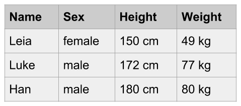
Figure 18.3: Data in tabular format

This is another example of raw data, in particular a raw data table. The data is visually organized and displayed in a rectangular grid of cells. However, this table is not ready yet to be manipulated statistically, much less algebraically. Obviously, this table needs some processing and cleaning in order to obtain a table with numerical information that becomes suitable for mathematical operations.

More often than not, raw data will be far from being in tabular format, or at least it will require extra reshaping steps so that it can be ready for the analysis. We hope that most of the content in the book will give you solid skills to get data in the right rectangular shape.

18.1.2 Tabular Data

Eventually, to be analyzed with statistical learning tools and other multivariate techniques, your data will typically be required to have a certain specific structure, usually in the form of some sort of table or spreadsheet format (e.g. rows and columns).

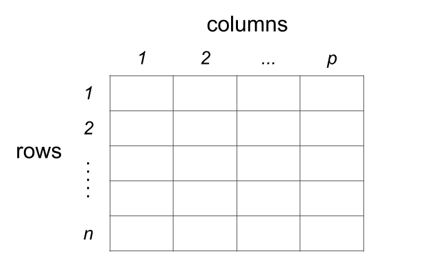
Figure 18.4: Data Table Format

Depending on the nature of the data, and the way it is organized, rows and columns will have a particular meaning. The most common data table setting is the one of individuals-and-variables. Although somewhat arbitrary, the standard convention is that we use the columns to represent variables, and the rows to represent individuals.

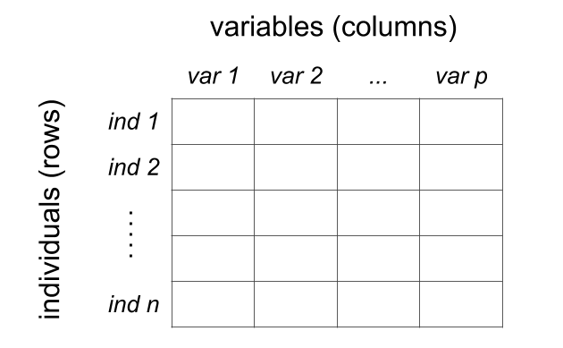
Figure 18.5: Conceptual table of individuals and variables

18.2 Types of Tables

The most typical table format is that of individuals (rows) and variables (columns). However, the individuals-variables layout is not the only type of setting; there are other types of tables like contingency tables, crosstabulations, distance tables, as well as similarity and proximity tables. So let’s review some examples of various kinds of rectangular formats.

18.2.1 Heterogeneous Table

Perhaps the most ubiquitous type of table is that of inidividuals and variables in which the variables represent mixed or heterogeneous information. The toy data introduced so far is an example of a heterogeneous table involving distinct flavors of variables such as Name, Sex, Hieght and Weight. In other words, Name and Sex have strings values or categories, while Height and Weight have numeric values (representing quantities).

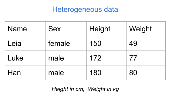
Figure 18.6: Mixed or heterogeneous variables

As you can tell, Height and Weight are already expressed in numeric values, and you can actually do some math on them (i.e. apply arithmetic and algebraic operations). In contrast, Name and Sex are not codified numerically, so the type of mathematical operations that you can perform on them is very limited. In order to exploit their information in a deeper sense, you would have to transform the categories male and female with some numeric coding.

18.2.2 Binary table

Another common type of table is a binary table. As its name indicates, this type of table contains variables that can only take two values. For example presence-absence, female-male, yes-no, success-failure, case-control, etc. In the table below, the variables represent drinks consumed: Beer, Wine, Juice, Coffee, and Tea. Each variable takes two possible values, yes and no, indicating whether an individual consumes a specific type of drink.

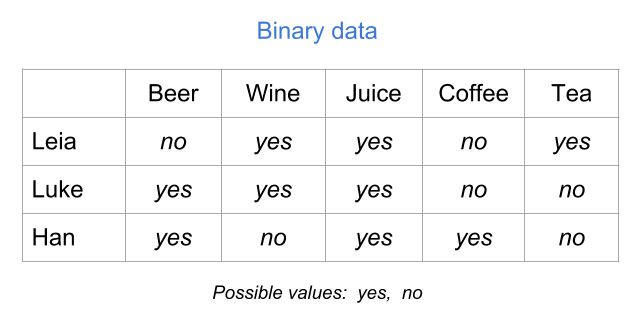
Figure 18.7: Binary table (raw values)

Although the values yes and no are very descriptive, you will need to encode them numerically to be able to perform statitical or algebraic operations with them. Perhaps the most natural way to encode binary values is with zeros and ones: “yes” = 1, and “no” = 0.

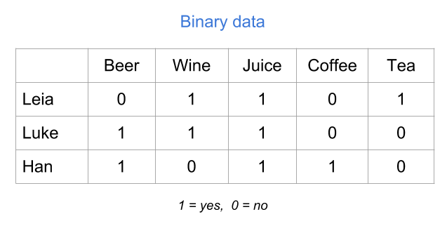
Figure 18.8: Binary table (numeric values)

Another possible codification could be “yes” = 1, and “no” = -1. Or also with logical values: “yes” = TRUE, and “no” = FALSE.

18.2.3 Modalities table

Another type of table consists of so-called modalities. These can come from variables or questions in a survey about how frequent you use/consume a specific product.

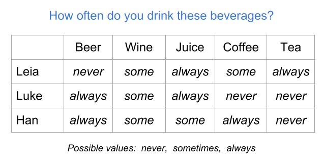
Figure 18.9: Table of modalities (raw values)

In order to statistically treat a modalities table, you will very likely have to transform the values of the categories (i.e. the modalities) to some numeric coding. For instance, you can assign values 1 = “never”, 2 = “sometimes”, and 3 = “always.”

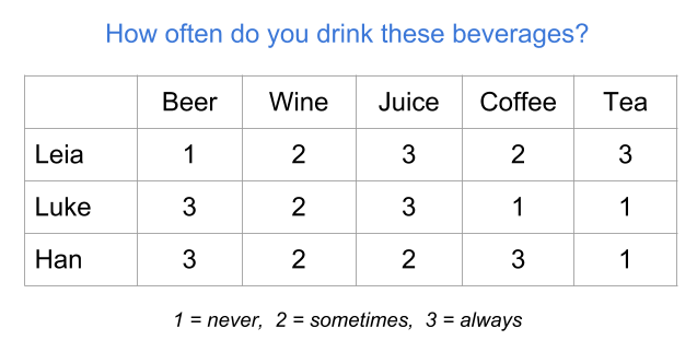
Figure 18.10: Table of modalities (numeric values)

18.2.4 Preference table

A preference table is a special case of individuals-variables table in which the variables are measured in some kind of preference scale. For example, we can measure the preference level for various types of fruit juices on an ordinal scale ranging from 1 = “don’t like at all” to 5 = “like it very much.”

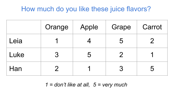
Figure 18.11: Table of frequencies

18.2.5 Frequency table

As its name suggests, this type of table contains the frequencies (i.e. counts) resulting from crossing two categorical variables. This is the reason why you also find the name cross-tables for this type of tabular data. Another common name for this type of tables is contingency table.

The example below shows a frequency table of the number of dialogues of each character, per episode (in the original trilogy of Star Wars). The rows correspond to the categories of the variable Name, while the columns corresponds to the categories of the variable Episode.

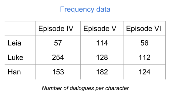
Figure 18.12: Table of frequencies

The value in the ij-th cell (i-th row, j-th column) tells you the number of occurrences that share Name’s category i and Episode’s category j. If you add all the entries, you get the total number of individuals in each variable.

This tabular format is not really an individuals-variables table. Even though the example above has rows with names of the three individuals, the way you get a table like this is with two categorical variables.

18.2.6 Distance table

Another interesting type of table is a distance table. Depending on who you talk to, the term “distance” may be used with slightly different meanings. Some authors refer to the word distance conveying a metric distance meaning. Other authors instead use the word distance to convey a general idea of dissimilarity.

In general, you can find distance tables under two opposite perspectives: similarities and disimilarities. The table below is an example of a similarity table.

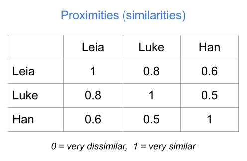
Figure 18.13: Table of proximities

18.2.7 Summary

• Most statistical learning methods require data in a table format with multiple columns and rows.

• It’s important to be aware of the difference between a raw data table, and a clean table numerically codified.

• For most of this book, we’ll consider a data set to be integrated by a group of individuals or objects on which we observe or measure one or more characteristics called variables.