23 Pipes and More dplyr
23.1 Introduction
In previous chapters, we started to manipulate data tables (e.g. data.frame,
tibble) with functions provided by the R package "dplyr".
Having been exposed to the dplyr paradigm, let’s compare R base manipulation against the various dplyr syntax flavors.
23.1.1 Starwars Data Set
In this tutorial we are going to use the data set starwars that comes in
"dplyr":
# data set
starwars
#> # A tibble: 87 x 13
#>    name  height  mass hair_color skin_color eye_color birth_year gender
#>    <chr>  <int> <dbl> <chr>      <chr>      <chr>          <dbl> <chr>
#>  1 Luke…    172    77 blond      fair       blue            19   male
#>  2 C-3PO    167    75 <NA>       gold       yellow         112   <NA>
#>  3 R2-D2     96    32 <NA>       white, bl… red             33   <NA>
#>  4 Dart…    202   136 none       white      yellow          41.9 male
#>  5 Leia…    150    49 brown      light      brown           19   female
#>  6 Owen…    178   120 brown, gr… light      blue            52   male
#>  7 Beru…    165    75 brown      light      blue            47   female
#>  8 R5-D4     97    32 <NA>       white, red red             NA   <NA>
#>  9 Bigg…    183    84 black      light      brown           24   male
#> 10 Obi-…    182    77 auburn, w… fair       blue-gray       57   male
#> # … with 77 more rows, and 5 more variables: homeworld <chr>, species <chr>,
#> #   films <list>, vehicles <list>, starships <list>
For illustration purposes, let’s consider a relatively simple example. Say we are interested in calculating the average (mean) height for both female and male individuals. Let’s discuss how to find the solution under the base R approach, as well as the dplyr approach.
23.2 Base R approach
Let’s see how to use base R operations to find the average height of
individuals with gender female and male.
# identify female and male individuals
# (comparison operations)
which_females <- starwars$gender == 'female'
which_males <- starwars$gender == 'male'
# select the height values of females and males
# (via logical subsetting)
height_females <- starwars$height[which_females]
height_males <- starwars$height[which_males]# calculate averages (removing missing values)
avg_ht_female <- mean(height_females, na.rm = TRUE)
avg_ht_male <- mean(height_males, na.rm = TRUE)
# optional: display averages in a vector
c('female' = avg_ht_female, 'male' = avg_ht_male)
#> female male
#> 165 179All the previous code can be written with more compact expressions:
23.3 With "dplyr"
The behavior of "dplyr" is functional in the sense that function calls don’t
have side-effects. You must always save their results in order to keep them
in an object (in memory). This doesn’t lead to particularly elegant code,
especially if you want to do many operations at once.
23.3.1 Option 1) Step-by-step
You either have to do it step-by-step:
# manipulation step-by-step
gender_height <- select(starwars, gender, height)
fem_male_height <- filter(gender_height,
                          gender == 'female' | gender == 'male')
height_by_gender <- group_by(fem_male_height, gender)
summarise(height_by_gender, mean(height, na.rm = TRUE))
#> # A tibble: 2 x 2
#>   gender `mean(height, na.rm = TRUE)`
#>   <chr>                         <dbl>
#> 1 female                         165.
#> 2 male                           179.
23.3.2 Option 2) Nested (embedded) code
Or if you don’t want to name the intermediate results, you need to wrap the function calls inside each other:
summarise(
  group_by(
    filter(select(starwars, gender, height),
           gender == 'female' | gender  == 'male'),
    gender),
  mean(height, na.rm = TRUE)
)
#> # A tibble: 2 x 2
#>   gender `mean(height, na.rm = TRUE)`
#>   <chr>                         <dbl>
#> 1 female                         165.
#> 2 male                           179.
This is difficult to read because the order of the operations is from inside to out. Thus, the arguments are a long way away from the function.
23.3.3 Option 3) Piping
To get around the problem of nesting functions, "dplyr" also provides the
%>% operator from the R package "magrittr".
What does the piper %>% do? Here’s a conceptual example:
x %>% f(y) turns into f(x, y) so you can use it to rewrite multiple
operations that you can read left-to-right, top-to-bottom.
Here’s how to use the piper to calculate the average height for female and male individuals:
avg_height_by_gender <- starwars %>%
  select(gender, height) %>%
  filter(gender == 'female' | gender == 'male') %>%
  group_by(gender) %>%
  summarise(avg = mean(height, na.rm = TRUE))
avg_height_by_gender
#> # A tibble: 2 x 2
#>   gender   avg
#>   <chr>  <dbl>
#> 1 female  165.
#> 2 male    179.
avg_height_by_gender$avg
#> [1] 165 179
Here’s another example in which we calculate the mean height and mean mass
of species Droid, Ewok, and Human; arranging the rows of the tibble by mean
height, in descending order:
starwars %>%
  select(species, height, mass) %>%
  filter(species %in% c('Droid', 'Ewok', 'Human')) %>%
  group_by(species) %>%
  summarise(
    mean_height = mean(height, na.rm = TRUE),
    mean_mass = mean(mass, na.rm = TRUE)
  ) %>%
  arrange(desc(mean_height))
#> # A tibble: 3 x 3
#>   species mean_height mean_mass
#>   <chr>         <dbl>     <dbl>
#> 1 Human          177.      82.8
#> 2 Droid          140       69.8
#> 3 Ewok            88       20
23.4 Pipes and Plots
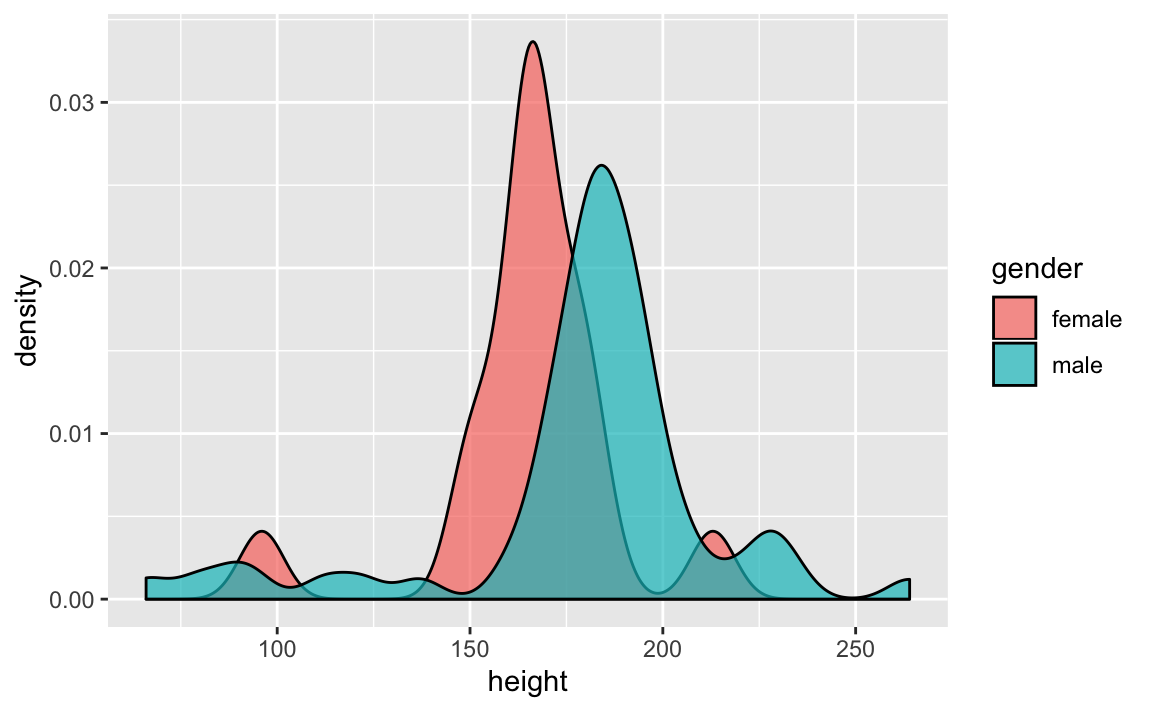
You can also the %>% operator to chain dplyr commands with ggplot commans
(and other R commands). The following examples combine some data manipulation
to filter() female and males individuals, in order to graph a density plot
of height
starwars %>%
  filter(gender %in% c('female', 'male')) %>%
  ggplot(aes(x = height, fill = gender)) +
  geom_density(alpha = 0.7)
#> Warning: Removed 5 rows containing non-finite values (stat_density).
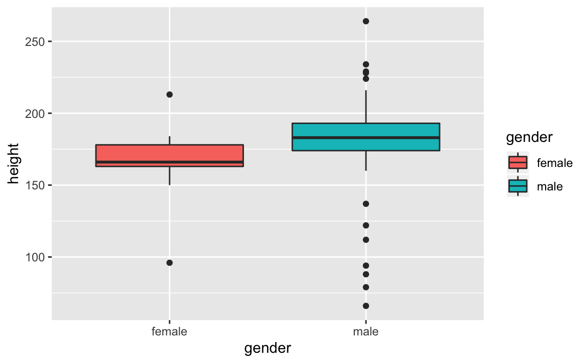
Here’s another example in which instead of graphing density plots, we graph
boxplots of height for female and male individuals:
starwars %>%
  filter(gender %in% c('female', 'male')) %>%
  ggplot(aes(x = gender, y = height, fill = gender)) +
  geom_boxplot()
#> Warning: Removed 5 rows containing non-finite values (stat_boxplot).
23.5 More Pipes
Often, you will work with functions that don’t take data frames (or tibbles) as
inputs. A typical example is the base plot() function used to produce a
scatterplot; you need to pass vectors to plot(), not data frames. In this
situations you might find the %$% operator extremely useful.
The %$% operator, also from the package "magrittr", is a cousin of the
%>% operator. What %$% does is to extract variables in a data frame
so that you can refer to them explicitly. Let’s see a quick example:
23.6 Exercises
Consider the following data frame dat
      first       last  gender     title  gpa
1       Jon       Snow    male      lord    3
2      Arya      Stark  female  princess    3
3    Tyrion  Lannister    male    master    4
4  Daenerys  Targaryen  female  khaleesi    3
5      Yara    Greyjoy  female  princess    4
1) What is the output of the following command?
dat %>%
  select(gender, gpa) %>%
  filter(gender == 'male') %>%
  summarise(max(gpa))
2) What is the output of the following command?
dat %>% select(first, last) %>% arrange(desc(first))3) What is the output of the following command?
dat %>%
  filter(gender == 'female' | title != 'khaleesi') %>%
  select(title)
Consider the following data frame dat
   Month  Week  Temp  Wind
1      5     1    67   7.4
2      5     2    72   8.0
3      5     3    74  12.6
4      5     4    62  11.5
5      6     1    78   8.6
6      6     2    74   9.7
7      6     3    67  16.1
8      6     4    84   9.2
4) What is the output of the following command? Try to guess the output without running the command.
5) What is the output of the following command? Try to guess the output without running the command.
Consider the following data frame dat
      first       last  gender     title  gpa
1       Jon       Snow    male      lord  3.0
2      Arya      Stark  female  princess  3.5
3    Tyrion  Lannister    male    master  4.0
4  Daenerys  Targaryen  female  khaleesi  3.8
5      Yara    Greyjoy  female  princess  1.5
6) Which of the following commands gives you the following output:
#>      first
#> 1     Yara
#> 2   Tyrion
#> 3      Jon
#> 4 Daenerys
#> 5     Arya
arrange(select(dat, first), desc(last))arrange(select(dat, first), first)arrange(select(dat, first), desc(first))- none of the above
7) Which of the following commands gives you the data of female individuals:
#>      first      last gender    title gpa
#> 1     Arya     Stark female princess 3.5
#> 2 Daenerys Targaryen female khaleesi 3.8
#> 3     Yara   Greyjoy female princess 1.5
filter(dat, gender == female)select(dat, gender == female)group_by(dat, gender == female)- none of the above
8) Which of the following commands gives you the following output:
#>   max(gpa)
#> 1 4which.max(dat$gpa)summarise(dat, max(gpa))max(dat$gpa)- none of the above