9.3 Correlation

Although the covariance indicates the direction—positive or negative—of a possible linear relation, it does not tell us how big or small the relation might be. To have a more interpretable index, we must transform the convariance into a unit-free measure. To do this we must consider the standard deviations of the variables so we can normalize the convariance. The result of this normalization is the coefficient of linear correlation defined as:

\[ cor(X, Y) = \frac{cov(X, Y)}{\sqrt{var(X)} \sqrt{var(Y)}} \]

Representing \(X\) and \(Y\) as vectors \(\mathbf{x}\) and \(\mathbf{y}\), we can express the correlation as:

\[ cor(\mathbf{x}, \mathbf{y}) = \frac{cov(\mathbf{x}, \mathbf{y})}{\sqrt{var(\mathbf{x})} \sqrt{var(\mathbf{y})}} \]

Assuming that \(\mathbf{x}\) and \(\mathbf{y}\) are mean-centered, we can express the correlation as:

\[ cor(\mathbf{x, y}) = \frac{\mathbf{x^\mathsf{T} y}}{\|\mathbf{x}\| \|\mathbf{y}\|} \]

As it turns out, the norm of a mean-centered variable \(\mathbf{x}\) is proportional to the square root of its variance (or standard deviation):

\[ \| \mathbf{x} \| = \sqrt{\mathbf{x^\mathsf{T} x}} = \sqrt{n} \sqrt{var(\mathbf{x})} \]

Consequently, we can also express the correlation with inner products as:

\[ cor(\mathbf{x, y}) = \frac{\mathbf{x^\mathsf{T} y}}{\sqrt{(\mathbf{x^\mathsf{T} x})} \sqrt{(\mathbf{y^\mathsf{T} y})}} \]

or equivalently:

\[ cor(\mathbf{x, y}) = \frac{\mathbf{x^\mathsf{T} y}}{\| \mathbf{x} \| \hspace{1mm} \| \mathbf{y} \|} \]

In the case that both \(\mathbf{x}\) and \(\mathbf{y}\) are standardized (mean zero and unit variance), that is:

\[ \mathbf{x} = \begin{bmatrix} \frac{x_1 - \bar{x}}{\sigma_{x}} \\ \frac{x_2 - \bar{x}}{\sigma_{x}} \\ \vdots \\ \frac{x_n - \bar{x}}{\sigma_{x}} \end{bmatrix}, \hspace{5mm} \mathbf{y} = \begin{bmatrix} \frac{y_1 - \bar{y}}{\sigma_{y}} \\ \frac{y_2 - \bar{y}}{\sigma_{y}} \\ \vdots \\ \frac{y_n - \bar{y}}{\sigma_{y}} \end{bmatrix} \]

the correlation is simply the inner product:

\[ cor(\mathbf{x, y}) = \mathbf{x^\mathsf{T} y} \hspace{5mm} \mathrm{(standardized} \hspace{1mm} \mathrm{variables)} \]

Let’s look at two variables (i.e. vectors) from a geometric perspective.

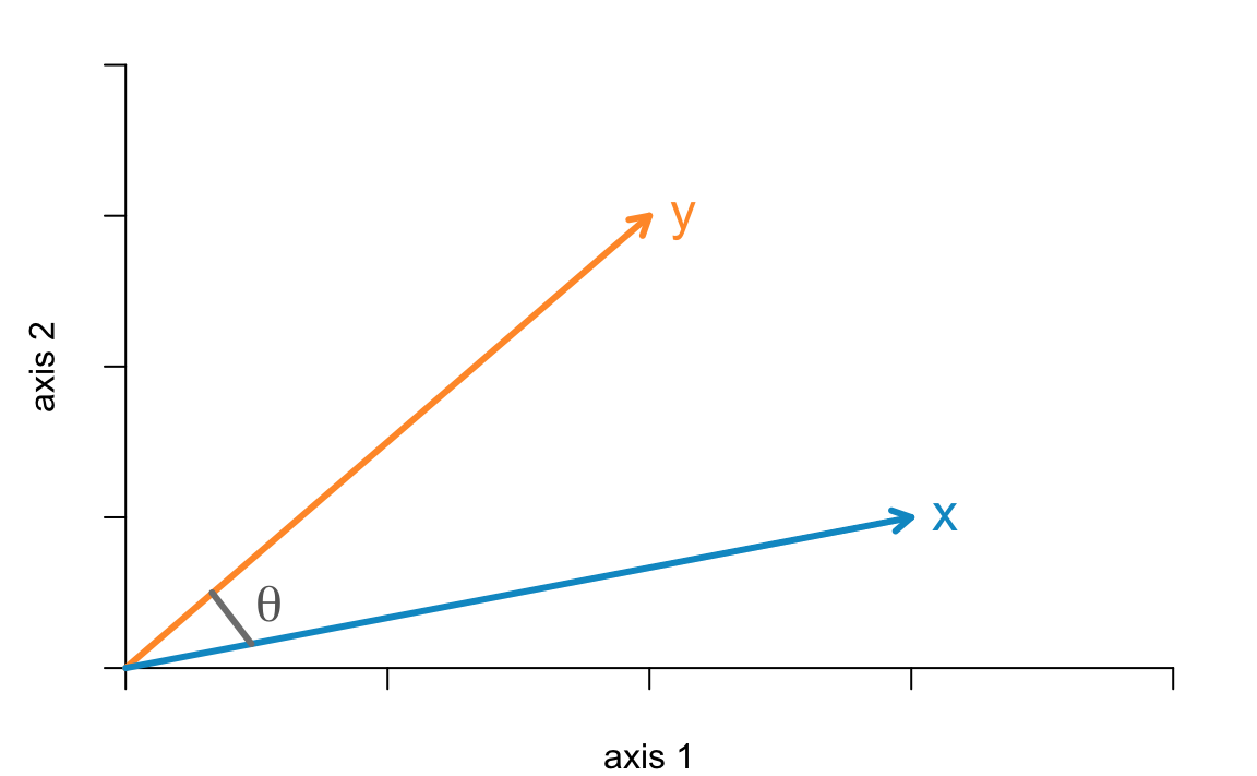
Figure 9.2: Two vectors in a 2-dimensional space

The inner product ot two mean-centered vectors \(\mathbf{x'y}\) is obtained with the following equation:

\[ \mathbf{x^\mathsf{T} y} = \|\mathbf{x}\| \|\mathbf{y}\| cos(\theta_{x,y}) \]

where \(cos(\theta_{x,y})\) is the angle between \(\mathbf{x}\) and \(\mathbf{y}\). Rearranging the terms in the previous equation we get that:

\[ cos(\theta_{x,y}) = \frac{\mathbf{x^\mathsf{T} y}}{\|\mathbf{x}\| \|\mathbf{y}\|} = cor(\mathbf{x, y}) \]

which means that the correlation between mean-centered vectors \(\mathbf{x}\) and \(\mathbf{y}\) turns out to be the cosine of the angle between \(\mathbf{x}\) and \(\mathbf{y}\).