2.2 Data Matrix
While the raw ingredient for any statistical learning endevour is a data set, typically reshaped and organized in a tabular form, the core input of any statistical learning method consists of the data matrix, or in some cases, matrices.
To make things less abstract I’m going to use the following toy data table with four variables measured on six individuals:
                  gender  height  weight      jedi
Anakin Skywalker    male    1.88    84.0  yes_jedi
Padme Amidala     female    1.65    45.0   no_jedi
Luke Skywalker      male    1.72    77.0  yes_jedi
Leia Organa       female    1.50    49.0   no_jedi
Qui-Gon Jinn        male    1.93    88.5  yes_jedi
Obi-Wan Kenobi      male    1.82    77.0  yes_jedi
You can actually find the corresponding CSV file in the data/ folder of the book’s github repository.
https://github.com/gastonstat/matrix4sl/blob/master/data/starwars.csv
2.2.1 Why a data matrix?
The reason to use matrices is simple: the typical structure in which the data can be mathematically manipulated from a multivariate standpoint is a data matrix. No other mathematical object adapts so well to the rectangular structure of a data table.
Since we are getting into more formal mathematical territory, we need to define some terminology and notation that we’ll use in the rest of the book.
We are going to represent matrices with bold upper-case letters like \(\mathbf{A}\) or \(\mathbf{B}\).
In general, a matrix \(\mathbf{X}\) has \(n\) rows and \(p\) columns, and we say that \(\mathbf{X}\) is an \(n \times p\) matrix. In addition, we are going to assume that all the matrices are real matrices, that is, matrices containing elements in the set of Real numbers.
\[ \underset{n \times p}{\mathbf{X}} = \left[\begin{array}{ccccc} x_{11} & \cdots & x_{1j} & \cdots & x_{1p} \\ \vdots & & \vdots & & \vdots \\ x_{i1} & \cdots & x_{ij} & \cdots & x_{ip} \\ \vdots & & \vdots & & \vdots \\ x_{n1} & \cdots & x_{nj} & \cdots & x_{np} \\ \end{array}\right] \]
An element of a matrix \(\mathbf{X}\) is denoted by \(x_{ij}\) which represents the element in the \(i\)-th row and the \(j\)-th column. For instance, the element \(x_{23}\) in our toy \(6 \times 4\) data matrix has the value 45 and it represents the weight of Padme Amidala.
Together with matrices we also have variables, and vectors. We are going to represent variables with italized capital letters such as \(Y\) and \(Z\). Also, variables in a matrix \(\mathbf{X}\) can be represented with subscripts such as \(X_j\) to indicate the column-index position. The first three variables in our matrix \(\mathbf{X}\) would be represented as \(X_1\) (gender), \(X_2\) (height), and \(X_3\) (weight).
Vectors will be represented by bold lower case letters such as \(\mathbf{w}\) or \(\mathbf{u}\). A vector \(\mathbf{w}\) with \(m\) elements can be expressed as \(\mathbf{w} = (w_1, w_2, \dots, w_m)\). Since variables can be expressed as vectors, we can use the vector notation \(\mathbf{x}\) to represent a variable \(X\). However, keep in mind that not all vectors are variables: a vector may well refer to an object or to any row of a matrix.
2.2.2 Matrix Representations
You will find that people represent matrices in multiple ways, using various notations, symbols, and diagrams.
We can represent a data matrix \(\mathbf{X}\) by simply regarding the matrix from its columns (i.e. variables) perspective:
\[ \mathbf{X} = \left[\begin{array}{c|c|c|c|c|c} & & & & & \\ \mathbf{x}_{1} & \mathbf{x}_{2} & \cdots & \mathbf{x}_{j} & \cdots & \mathbf{x}_{p} \\ & & & & & \\ \end{array}\right] \]
Note that each variable \(X_j\) is represented with a column vector \(\mathbf{x}_{j}\). In turn, the vertical lines are just a visual cue indicating separation between columns. Taking our toy data data matrix, we could represent it as:
\[ \mathbf{Data} = \left[\begin{array}{c|c|c|c} & & & \\ \texttt{gender} & \texttt{height} & \texttt{weight} & \texttt{jedi} \\ & & & \\ \end{array}\right] \]
Being more minimalists, we can even get a more compact representation by just expressing a matrix \(\mathbf{X}\) as a list or sequence of its variables:
\[ \mathbf{X} = \left[\begin{array}{cccccc} \mathbf{x}_{1} & \mathbf{x}_{2} & \cdots & \mathbf{x}_{j} & \cdots & \mathbf{x}_{p} \\ \end{array}\right] \]
2.2.3 A Block of Variables
While most of us are used to think of multivariate data in terms of a table or matrix, there can be other interesting representation options. If you are like me who loves to visualize concepts, we can also use an alternative way to display the variables using a standard convention of drawing them in rectangular shape. In this way, we can depict a set of variables in a data matrix as a series of rectangles, like those below inside the dashed box:
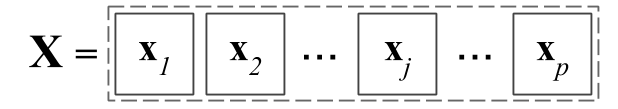
Figure 2.1: Variables in a matrix depicted as a set of rectangles
The rectangular-box shape perfectly illustrates the idea of a block of variables. I will use the term block to convey the idea of a group or set of variables measured on a set of objects. If you prefer, you can also think of a block as a data table.