1.2 Types of Tables
The most typical table format is that of individuals (rows) and variables (columns). However, the individuals-variables layout is not the only type of setting; there are other types of tables like contingency tables, crosstabulations, distance tables, as well as similarity and proximity tables. So let’s review some examples of various kinds of rectangular formats.
1.2.1 Heterogeneous Table
Perhaps the most ubiquitous type of table is that of inidividuals and variables in which the variables represent mixed or heterogeneous information. The toy data introduced so far is an example of a heterogeneous table involving distinct flavors of variables such as Name, Sex, Hieght and Weight. In other words, Name and Sex have strings values or categories, while Height and Weight have numeric values (representing quantities).
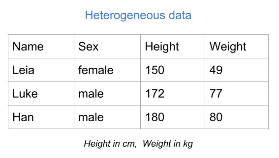
Figure 1.6: Mixed or heterogeneous variables
As you can tell, Height and Weight are already expressed in numeric values, and you can actually do some math on them (i.e. apply arithmetic and algebraic operations). In contrast, Name and Sex are not codified numerically, so the type of mathematical operations that you can perform on them is very limited. In or der to exploit their information in a deeper sense, you would have to transform the categories male and female with some numeric coding.
1.2.2 Binary table
Another common type of table is a binary table. As its name indicates, this type of table contains variables that can only take two values. For example presence-absence, female-male, yes-no, success-failure, case-control, etc. In the table below, the variables represent drinks consumed: Beer, Wine, Juice, Coffee, and Tea. Each variable takes two possible values, yes and no, indicating whether an individual consumes a specific type of drink.
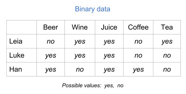
Figure 1.7: Binary table (raw values)
Although the values yes and no are very descriptive, you will need to codify them numerically to be able to perform statitical or algebraic operations with them. Perhaps the most natural way to codify binary values is with zeros and ones: “yes” = 1, and “no” = 0.
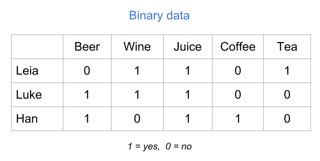
Figure 1.8: Binary table (numeric values)
Another possible codification could be “yes” = 1, and “no” = -1. Or also with logical values: “yes” = TRUE, and “no” = FALSE.
1.2.3 Modalities table
Another type of table consists of so-called modalities. These can come from variables or questions in a survey about how frequent you use/consume a specific product.
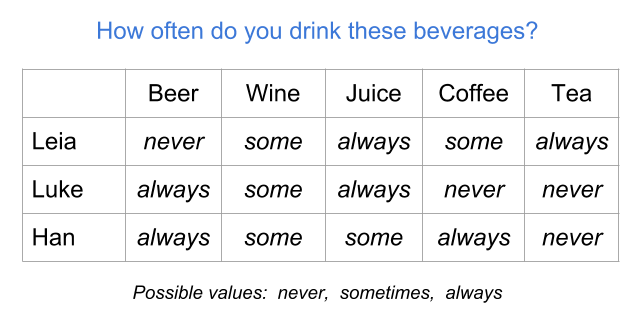
Figure 1.9: Table of modalities (raw values)
In order to statistically treat a modalities table, you will very likely have to transform the values of the categories (i.e. the modalities) to some numeric coding. For instance, you can assign values 1 = “never”, 2 = “sometimes”, and 3 = “always.”
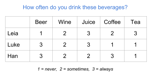
Figure 1.10: Table of modalities (numeric values)
1.2.4 Preference table
A preference table is a special case of individuals-variables table in which the variables are measured in some kind of preference scale. For example, we can measure the preference level for various types of fruit juices on an ordinal scale ranging from 1 = “don’t like at all” to 5 = “like it very much.”
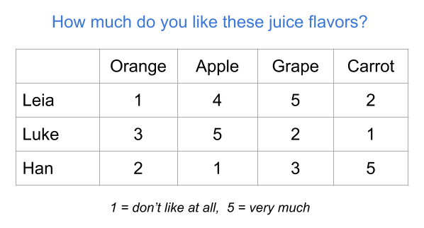
Figure 1.11: Table of frequencies
1.2.5 Frequency table
As its name suggests, this type of table contains the frequencies (i.e. counts) resulting from crossing two categorical variables. This is the reason why you also find the name cross-tables for this type of tabular data. Another common name for this type of tables is contingency table.
The example below shows a frequency table of the number of dialogues of each character, per episode (in the original trilogy of Star Wars). The rows correspond to the categories of the variable Name, while the columns corresponds to the categories of the variable Episode.
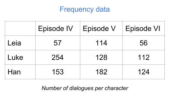
Figure 1.12: Table of frequencies
The value in the ij-th cell (i-th row, j-th column) tells you the number of occurrences that share Name’s category i and Episode’s category j. If you add all the entries, you get the total number of individuals in each variable.
This tabular format is not really an individuals-variables table. Even though the example above has rows with names of the three individuals, the way you get a table like this is with two categorical variables.
1.2.6 Distance table
Another interesting type of table is a distance table. Depending on who you talk to, the term “distance” may be used with slightly different meanings. Some authors refer to the word distance conveying a metric distance meaning. Other authors instead use the word distance to convey a general idea of dissimilarity.
In general, you can find distance tables under two opposite perspectives: similarities and disimilarities. The table below is an example of a similarity table.
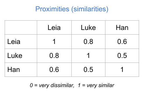
Figure 1.13: Table of proximities
1.2.7 Summary
Most statistical learning methods require data in a table format with multiple columns and rows.
It’s important to be aware of the difference between a raw data table, and a clean table numerically codified.
Unless otherwise specified, in this book we’ll assume that all the variables in a data matrix have numerical variables.
For most of this book, we’ll consider a data set to be integrated by a group of individuals or objects on which we observe or measure one or more characteristics called variables.
Make a donation
If you find this resource useful, please consider making a one-time donation in any amount. Your support really matters.