11.1 Decompositions

Simply put, decompositions are like factorizations of numbers. For example, consider the number 6; we can decompose 6 as the product of 3 and 2:

\[ 6 = 3 \times 2 \]

that is, we factorize 6 in terms of “simpler” numbers.

If the idea of factorizing numbers seems too simplistic to you, then consider the factorization of polynomials. Here’s one toy example with the following polynomial:

\[ p(x) = x^2 + 5x + 6 \]

The above quadratic polynomial can be decomposed as the product of two linear—and therefore more basic—polynomials:

\[ x^2 + 5x + 6 = (x + 3) (x + 2) \]

This factorization allows us to dismantle the quadratic polynomial into a product of polynomials of smaller degree. In particular, we observe that the two resulting terms contain the roots of the original polynomial: 3 and 2.

The same idea applies to matrix decompositions: they allow us to break down a matrix and decompose it in its main parts. They make it easier to study the properties of matrices, and they tend to make matrix computations easier.

11.1.1 General Idea

More formally, a matrix decomposition is a way of expressing a matrix \(\mathbf{M}\) as the product of a set of new—typically two or three—matrices, usually simpler in some sense, that gives us an idea of the inherent structures or relationships in \(\mathbf{M}\). By “simpler” we mean a series of ideas such as more compact matrices, or with less dimensions, or with less number of rows, or less number of columns; perhaps triangular matrices, or even matrices almost full of zeros, except in their diagonal.

Roughly speaking, the decomposition of an \(n \times p\) matrix \(\mathbf{M}\) can be described by a generic equation of the form:

\[ \mathbf{M} = \mathbf{A B C} \]

where the dimensions of the matrices are as follows:

• \(\mathbf{M}\) is \(n \times p\) (we assume for simplicity that \(n > p\))
• \(\mathbf{A}\) is \(n \times k\) (usually \(k < p\))
• \(\mathbf{B}\) is \(k \times k\) (usually diagonal)
• \(\mathbf{C}\) is \(k \times p\)

The following figure illustrates a matrix decomposition from the point of view of matrix shapes:

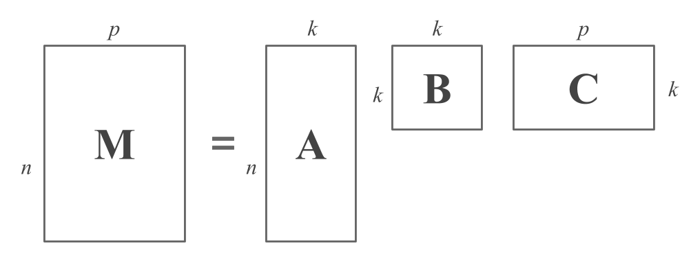
Figure 11.1: Matrix Decomposition Diagram

As you can tell, the matrix \(\mathbf{A}\) has the same number of rows as \(\mathbf{M}\). This is not a coincidence. In fact, each of the rows in \(\mathbf{A}\) provides information about the object described by the corresponding row of \(\mathbf{M}\). In this sense, the \(i\)-th row of \(\mathbf{A}\) involves \(k\) bits of information that shed light on the data of the \(i\)-th object.

The matrix \(\mathbf{C}\) has the same number of columns as \(\mathbf{M}\). In the same way that \(\mathbf{A}\) has to do with the rows of \(\mathbf{M}\), the matrix \(\mathbf{C}\) has to do with the columns of \(\mathbf{M}\). Each column of \(\mathbf{C}\) gives a different perspective of the variable described by the corresponding column of \(\mathbf{M}\), in terms of \(k\) bits of information.

Observe that the common element in matrices \(\mathbf{A}\) and \(\mathbf{C}\) is previsely the constant \(k\). The role of \(k\) is to coerce a more comptact representation for the data as compared to its original form. While \(k = p\) might give a reasonable factorization, often \(k\) is chosen to be smaller than \(p\). We do this under the assumption that using less dimensions will still capture the intrinsic patterns in the data that might not be evident by direct inspection of \(\mathbf{M}\).

What about the middle matrix \(\mathbf{B}\)? This matrix cements the connections between the pieces of information i\(\mathbf{A}\) and \(\mathbf{C}\). Unless stated otherwise, we will assume that \(\mathbf{B}\) is diagonal. Now, keep in mind that some decompositions do not explicitly include this middle matrix. When that’s the case, we can always suppose the existance of a \(k \times k\) identity matrix \(\mathbf{I}\) such that we still get the general decomposition given by three matrices:

\[ \mathbf{M} = \mathbf{AC} = \mathbf{A I C} \]

11.1.2 Some Comments

The equation that describes a decomposition:

\[ \mathbf{M} = \mathbf{A B C} \]

does not explain how to compute one, or how such decomposition can reveal the structures implicit in a data matrix. Nowadays, the computation of a matrix decomposition is straightforward; software to compute each one is readily available, and understanding how the algorithms work is not necessary to be able to interpret the results.

Seeing how a matrix decomposition reveals structure in a dataset is more complicated. Each decomposition reveals a different kind of implicit structure and, for each decomposition, there are various ways to interpret the results.

There are many different types of matrix decompositions, and each of them reveal different kinds of underlying structure. We are going to focus our discussion on two of them:

1. the Singular Value Decomposition (SVD), and

2. the Eigen Value Decomposition (EVD).

Why these two decompositions? Because we concentrate on the two types of matrices more important in statistics: general rectangular matrices used to represent data tables, and positive semi-definite matrices used to represent covariance matrices, correlation matrices, and any matrix that results from a crossproduct.