13.2 SVD Rank-Reduction Theorem

A very interesting and alternative way to represent the SVD is with the following formula:

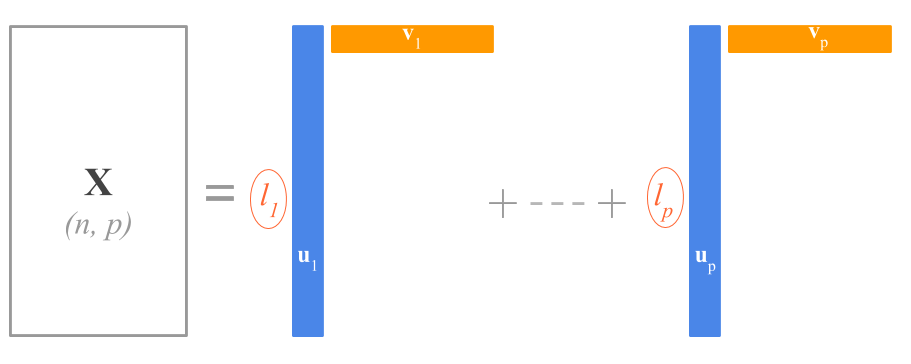
\[ \mathbf{X} = \sum_{k=1}^{p} l_k \mathbf{u_k} \mathbf{v^\mathsf{T}_k} \]

This equation expresses the SVD as a sum of \(p\) rank 1 matrices. This result is formalized in what is known as the SVD theorem described by Carl Eckart and Gale Young in 1936, and it is often referred to as the Eckart-Young theorem. This theorem applies to practically any arbitrary rectangular matrix.

The SVD theorem of Eckart and Young is related to the important problem of approximating a matrix. The basic result says that if \(\mathbf{X}\) is an \(n \times p\) rectangular matrix, then the best \(r\)-dimensional approximation \(\hat{\mathbf{X}}\) to \(\mathbf{X}\) is obtained by minimizing:

\[ min \| \mathbf{X - \hat{X}} \|^2 \]

This type of approximation is a least squares approximation and the solution is obtained by taking the first \(r\) elements of matrices \(\mathbf{U}, \mathbf{D}, \mathbf{V}\) so that the \(n \times r\) matrix

\[ \mathbf{\hat{X} = U_r D_r V^\mathsf{T}_r} \]

The SVD theorem says that any rectangular matrix \(\mathbf{X}\) can be broken down into the product of three matrices—an orthogonal matrix \(\mathbf{U}\), a diagonal matrix \(\mathbf{D}\), and the transpose of an orthogonal matrix \(\mathbf{V}\).

In terms of the diagonal elements \(l_1, l_2, \dots, l_r\) of \(\mathbf{D}\), the columns \(\mathbf{u_1}, \dots, \mathbf{u_r}\) of \(\mathbf{U}\), and the columns \(\mathbf{v_1}, \dots, \mathbf{v_r}\) of \(\mathbf{V}\), the basic structure of \(\mathbf{X}\) may be written as

\[ \mathbf{X} = l_1 \mathbf{u_1 v^\mathsf{T}_1} + l_2 \mathbf{u_2 v^\mathsf{T}_2} + \dots + l_r \mathbf{u_r v^\mathsf{T}_r} \]

which shows that the matrix \(\mathbf{X}\) of rank \(r\) is a linear combination of \(r\) matrices of rank 1.

Figure 13.3: SVD as a sum of rank-one matrices

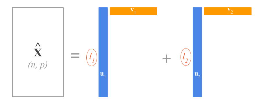
For eample, if you take only the first two singular vectors and values, you can obtain a two-rank approximation \(\mathbf{\hat{X}}\) of \(\mathbf{X}\).

\[ \mathbf{X} \approx \mathbf{\hat{X}_{2}} = l_1 \mathbf{u_1} \mathbf{v^\mathsf{T}_1} + l_2 \mathbf{u_2} \mathbf{v^\mathsf{T}_2} \]

Figure 13.4: SVD rank-two approximation

If you think about it, the SVD is of great utility because it tells us that the best 1-rank approximation, in the least squares sense, of any matrix \(\mathbf{X}\) is \(l_1 \mathbf{u_1} \mathbf{v^\mathsf{T}_1}\).

\[ \mathbf{X} \approx \mathbf{\hat{X}_1} = l_1 \mathbf{u_1} \mathbf{v^\mathsf{T}_1} \]

This implies that, from a conceptual standpoint, we can approximate the \(n \times p\) numbers in \(\mathbf{X}\) with just \(n + p + 1\) values: \(n\) numbers in \(\mathbf{u_1}\), \(p\) numbers in \(\mathbf{v_1}\), and one scalar \(l_1\).