13.1 SVD Basics
The Singular Value Decomposition expresses any matrix, such as an \(n \times p\) matrix \(\mathbf{X}\), as the product of three other matrices:
\[ \mathbf{X = U D V^\mathsf{T}} \]
where:
\(\mathbf{U}\) is a \(n \times p\) column orthonormal matrix containing the left singular vectors.
\(\mathbf{D}\) is a \(p \times p\) diagonal matrix containing the singular values of \(\mathbf{X}\).
\(\mathbf{V}\) is a \(p \times p\) column orthonormal matrix containing the right singular vectors.
In terms of the shapes of the matrices, the SVD decomposition has this form:
\[ \begin{bmatrix} & & \\ & & \\ & \mathbf{X} & \\ & & \\ & & \\ \end{bmatrix} = \ \begin{bmatrix} & & \\ & & \\ & \mathbf{U} & \\ & & \\ & & \\ \end{bmatrix} \ \begin{bmatrix} & & \\ & \mathbf{D} & \\ & & \\ \end{bmatrix} \ \begin{bmatrix} & & \\ & \mathbf{V}^\mathsf{T} & \\ & & \\ \end{bmatrix} \]
The SVD says that we can factorize \(\mathbf{X}\) with the product of an orthonormal matrix \(\mathbf{U}\), a diagonal matrix \(\mathbf{D}\), and an orthonormal matrix \(\mathbf{V}\).
\[ \mathbf{X} = \ \begin{bmatrix} u_{11} & \cdots & u_{1p} \\ u_{21} & \cdots & u_{2p} \\ \vdots & \ddots & \vdots \\ u_{n1} & \cdots & u_{np} \\ \end{bmatrix} \ \begin{bmatrix} l_{1} & \cdots & 0 \\ \vdots & \ddots & \vdots \\ 0 & \cdots & l_{p} \\ \end{bmatrix} \ \begin{bmatrix} v_{11} & \cdots & v_{p1} \\ \vdots & \ddots & \vdots \\ v_{1p} & \cdots & v_{pp} \\ \end{bmatrix} \]
13.1.1 SVD Properties
You can think of the SVD structure as the basic structure of a matrix. What does this mean? Well, to understand the meaning of basic structure, we need to say more things about what each of the matrices \(\mathbf{U}\), \(\mathbf{D}\), and \(\mathbf{V}\) represent. To be more precise:
About \(\mathbf{U}\)
The matrix \(\mathbf{U}\) is the orthonormalized matrix which is the most basic component. It’s like the skeleton of the matrix.
- \(\mathbf{U}\) is unitary, and its columns form a basis for the space spanned by the columns of \(\mathbf{X}\).
\[ \mathbf{U^\mathsf{T} U} = \mathbf{I}_{p} \]
- \(\mathbf{U}\) cannot be orthogonal (\(\mathbf{U U^\mathsf{T} = I_n}\)) unless \(r = p\)
About \(\mathbf{V}\)
The matrix \(\mathbf{V}\) is the orientation or correlational component.
- \(\mathbf{V}\) is unitary, and its columns form a basis for the space spanned by the rows of \(\mathbf{X}\).
\[ \mathbf{V^\mathsf{T} V} = \mathbf{I}_{p} \]
- \(\mathbf{V}\) cannot be orthogonal (\(\mathbf{V V^\mathsf{T} = I_p}\)) unless \(r = p = m\)
About \(\mathbf{D}\)
The matrix \(\mathbf{D}\) is referred to as the spectrum and it is a scale component. Note that all the values in the diagonal of \(\mathbf{D}\) are non-negative numbers.
This matrix is also unique. It is a like a fingerprint of a matrix. It is assumed that the singular values are ordered from largest to smallest.
All elements of \(\mathbf{D}\) can be taken to be positive, ordered from large to small (with ties allowed).
\(\mathbf{D}\) has non-negative real numbers on the diagonal (assuming \(\mathbf{X}\) is real).
The rank of \(\mathbf{X}\) is given by \(r\), the number of such positive values (which are called singular values). Furthermore, \(r(\mathbf{X}) \leq min(n,p)\).
13.1.2 Diagrams of SVD
Under the standard convention that \(n > p\), if we assume that \(\mathbf{X}\) is of full-column rank \(r(\mathbf{X}) = p\), then we can display the decomposition with the following diagram:
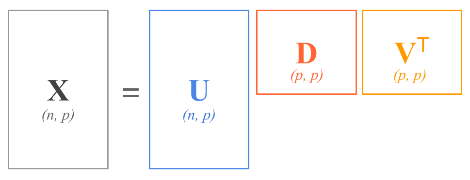
Figure 13.1: SVD Decomposition Diagram
In general, when the decomposed matrix \(\mathbf{X}\) is not of full column-rank, that is \(rank(\mathbf{X}) = r < p\), then the diagram of SVD could be depicted as follows
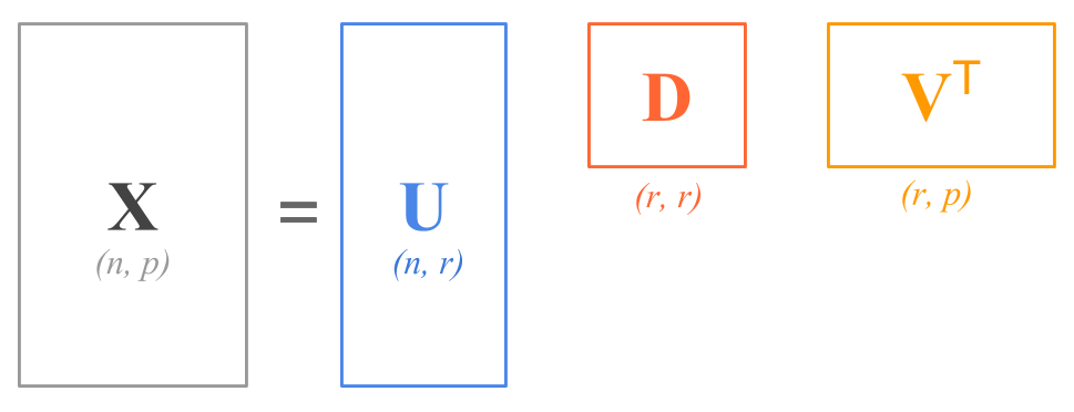
Figure 13.2: SVD Decomposition Diagram
13.1.3 Example
Here’s an example of SVD in R, via the function svd(). First let’s create a matrix \(\mathbf{X}\) with random numbers:
# X matrix
set.seed(22)
X <- matrix(rnorm(20), 5, 4)
X
       [,1]   [,2]   [,3]   [,4]
[1,] -0.512  1.858 -0.764 -0.922
[2,]  2.485 -0.066  0.082  0.862
[3,]  1.008 -0.163  0.743  2.003
[4,]  0.293 -0.200 -0.084  0.937
[5,] -0.209  0.301 -0.793 -1.616
R comes with the function svd(); it’s output is a list with three elements:
# singular value decomposition
SVD <- svd(X)

# elements returned by svd()
names(SVD)
[1] "d" "u" "v"dis a vector containing the singular values (i.e. values in the diagonal of \(\mathbf{D}\))uis the matrix of left singular values.vis the matrix of right singular values.
# vector of singular values
(d <- SVD$d)
[1] 3.952 2.022 1.475 0.432

# matrix of left singular vectors
(U = SVD$u)
       [,1]    [,2]   [,3]     [,4]
[1,] -0.425 -0.5391 -0.723  0.00979
[2,]  0.527 -0.7686  0.286  0.05610
[3,]  0.575  0.0500 -0.442  0.13107
[4,]  0.222  0.0527 -0.170 -0.95123
[5,] -0.402 -0.3366  0.413 -0.27337

# matrix of right singular vectors
(V = SVD$v)
       [,1]   [,2]    [,3]   [,4]
[1,]  0.571 -0.741  0.3386  0.104
[2,] -0.274 -0.530 -0.7680  0.234
[3,]  0.277  0.321 -0.0446  0.905
[4,]  0.723  0.261 -0.5418 -0.341
Let’s check that \(\mathbf{X} = \mathbf{U D V^\mathsf{T}}\)
# X equals U D V'
U %*% diag(d) %*% t(V)
       [,1]   [,2]   [,3]   [,4]
[1,] -0.512  1.858 -0.764 -0.922
[2,]  2.485 -0.066  0.082  0.862
[3,]  1.008 -0.163  0.743  2.003
[4,]  0.293 -0.200 -0.084  0.937
[5,] -0.209  0.301 -0.793 -1.616

# compare to X
X
       [,1]   [,2]   [,3]   [,4]
[1,] -0.512  1.858 -0.764 -0.922
[2,]  2.485 -0.066  0.082  0.862
[3,]  1.008 -0.163  0.743  2.003
[4,]  0.293 -0.200 -0.084  0.937
[5,] -0.209  0.301 -0.793 -1.616
Let’s also confirm that \(\mathbf{U}\) and \(\mathbf{V}\) are orthonormal:
# U orthonormal  (U'U = I)
t(U) %*% U
         [,1]      [,2]      [,3]      [,4]
[1,] 1.00e+00  1.39e-16  2.78e-17  0.00e+00
[2,] 1.39e-16  1.00e+00 -2.78e-17 -8.33e-17
[3,] 2.78e-17 -2.78e-17  1.00e+00  5.55e-17
[4,] 0.00e+00 -8.33e-17  5.55e-17  1.00e+00

# V orthonormal  (V'V = I)
t(V) %*% V
          [,1]      [,2]      [,3]      [,4]
[1,]  1.00e+00 -1.11e-16 -5.55e-17  1.11e-16
[2,] -1.11e-16  1.00e+00  8.33e-17  1.94e-16
[3,] -5.55e-17  8.33e-17  1.00e+00 -8.33e-17
[4,]  1.11e-16  1.94e-16 -8.33e-17  1.00e+00
13.1.4 Relation of SVD and Cross-Product Matrices
If you consider \(\mathbf{X}\) to be a data matrix of \(n\) individuals and \(p\) variables, you should be able to recall that we can obtain two cross-products: \(\mathbf{X^\mathsf{T}X}\) and \(\mathbf{X X^\mathsf{T}}\). It turns out that we can use the singular value decomposition of \(\mathbf{X}\) to find the corresponding factorization of each of these products.
The cross-product matrix of columns can be expressed as:
\[\begin{align*} \mathbf{X^\mathsf{T} X} &= (\mathbf{U D V^\mathsf{T}})^\mathsf{T} (\mathbf{U D V^\mathsf{T}}) \\ &= (\mathbf{V D U^\mathsf{T}}) (\mathbf{U D V^\mathsf{T}}) \\ &= \mathbf{V D} (\mathbf{U^\mathsf{T}} \mathbf{U}) \mathbf{D V^\mathsf{T}} \\ &= \mathbf{V D^2 V^\mathsf{T}} \end{align*}\]
The cross-product matrix of rows can be expressed as:
\[\begin{align*} \mathbf{X X^\mathsf{T}} &= (\mathbf{U D V^\mathsf{T}}) (\mathbf{U D V^\mathsf{T}})^\mathsf{T} \\ &= (\mathbf{U D V^\mathsf{T}}) (\mathbf{V D U^\mathsf{T}}) \\ &= \mathbf{U D} (\mathbf{V^\mathsf{T}} \mathbf{V}) \mathbf{D U^\mathsf{T}} \\ &= \mathbf{U D^2 U^\mathsf{T}} \end{align*}\]
One of the interesting things about SVD is that \(\mathbf{U}\) and \(\mathbf{V}\) are matrices whose columns are eigenvectors of product moment matrices that are derived from \(\mathbf{X}\). Specifically,
\(\mathbf{U}\) is the matrix of eigenvectors of (symmetric) \(\mathbf{XX^\mathsf{T}}\) of order \(n \times n\)
\(\mathbf{V}\) is the matrix of eigenvectors of (symmetric) \(\mathbf{X^\mathsf{T}X}\) of order \(p \times p\)
Of additional interest is the fact that \(\mathbf{D}\) is a diagonal matrix whose main diagonal entries are the square roots of \(\mathbf{U}^2\), the common matrix of eigenvalues of \(\mathbf{XX^\mathsf{T}}\) and \(\mathbf{X^\mathsf{T}X}\).
The EVD of the cross-product matrix of columns (or minor product moment) \(\mathbf{X^\mathsf{T} X}\) can be expressed as:
\[ \mathbf{X^\mathsf{T} X} = \mathbf{V \Lambda V^\mathsf{T}} \]
in terms of the SVD factorization of \(\mathbf{X}\):
\[ \mathbf{X^\mathsf{T} X} = \mathbf{V D^2 V^\mathsf{T}} \]
The EVD of the cross-product matrix of rows (or major product moment) \(\mathbf{X X^\mathsf{T}}\) can be expressed as:
\[ \mathbf{X X^\mathsf{T}} = \mathbf{U \Lambda U^\mathsf{T}} \]
in terms of the SVD factorization of \(\mathbf{X}\):
\[ \mathbf{X X^\mathsf{T}} = \mathbf{U D^2 U^\mathsf{T}} \]