9.4 Relation as Linear Approximation
A linked but different way to examine relations between the variables is when we ask: Can we approximate one of the variables in terms of the other? This is an asymmetric type of association since we seek to say something about the variability of one variable, say \(\mathbf{y}\), in terms of the variability of \(\mathbf{x}\).
We can think of several ways to approximate \(\mathbf{y}\) in terms of \(\mathbf{x}\). The approximation of \(\mathbf{y}\), denoted by \(\hat{\mathbf{y}}\), means finding a coefficient \(b\) such that:
\[ \hat{\mathbf{y}} = b \mathbf{x} \]
The common approach to get \(\hat{\mathbf{y}}\) in some optimal way is by minimizing the square difference between \(\mathbf{y}\) and \(\hat{\mathbf{y}}\).
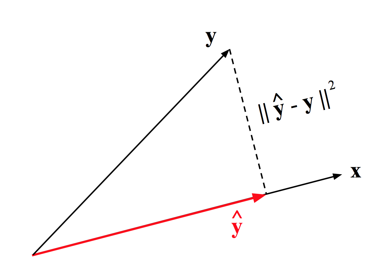
Figure 9.3: Linear approximation
The answer to this question comes in the form of a projection. More precisely, we orthogonally project \(\mathbf{y}\) onto \(\mathbf{x}\):
\[ \hat{\mathbf{y}} = \mathbf{x} \left( \frac{\mathbf{y^\mathsf{T} x}}{\mathbf{x^\mathsf{T} x}} \right) \]
or equivalently:
\[ \hat{\mathbf{y}} = \mathbf{x} \left( \frac{\mathbf{y^\mathsf{T} x}}{\| \mathbf{x} \|^2} \right) \]
Note that the term in parenthesis is just a scalar, so we can actually express \(\hat{\mathbf{y}}\) as \(b \mathbf{x}\). This means that a projection implies multiplying \(\mathbf{x}\) by some number \(b\), such that \(\hat{\mathbf{y}} = b \mathbf{x}\) is a stretched or shrinked version of \(\mathbf{x}\). This is nothing else than the least squares regression of \(\mathbf{y}\) on \(\mathbf{x}\). This is better appreciated in the following figure.
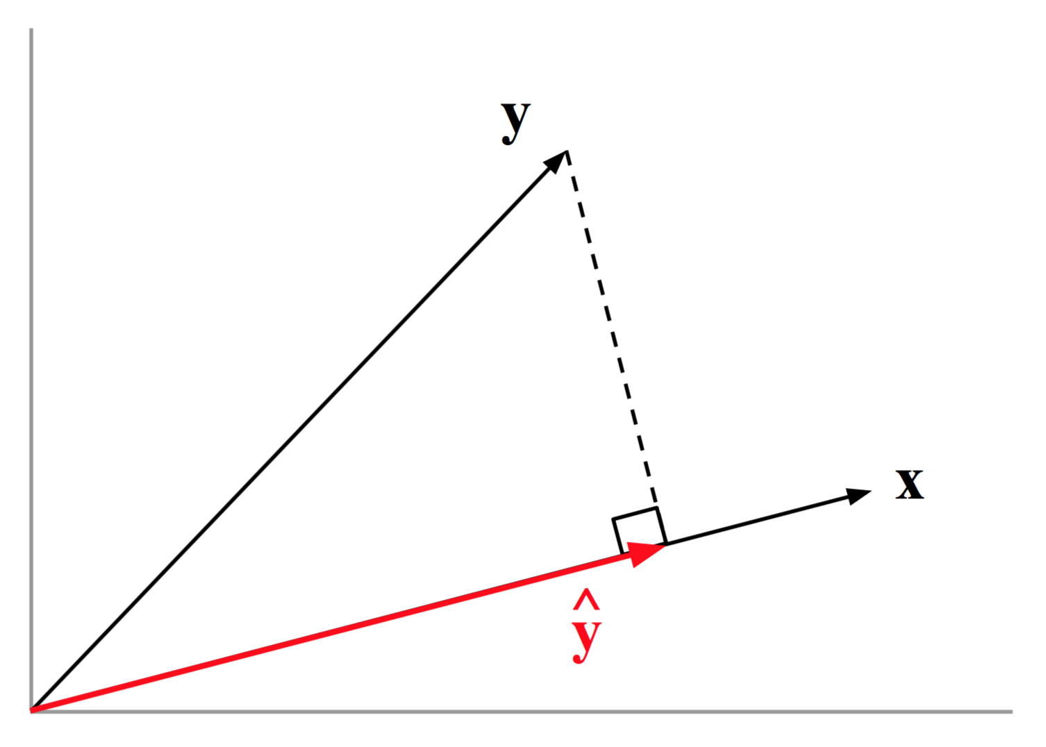
Figure 9.4: Orthogonal projection
Note that the correlation between \(\mathbf{y}\) and \(\hat{\mathbf{y}}\) is:
\[ cor(\mathbf{y}, \hat{\mathbf{y}}) = \frac{\mathbf{y^\mathsf{T} x}}{\| \mathbf{y} \|} \]
or alternatively:
\[ cor^{2}(\mathbf{y}, \hat{\mathbf{y}}) = \frac{\mathbf{y^\mathsf{T} x}}{\mathbf{y^\mathsf{T}}y} \]