12.3 Power Method

Among all the set of methods which can be used to find eigenvalues and eigenvectors, one of the basic procedures following a successive approximation approach is the so-called Power Method.

In its simplest form, the Power Method (PM) allows us to find the largest eigenvector and its corresponding eigenvalue. To be more precise, the PM allows us to find an approximation for the first eigenvalue of a symmetric matrix \(\mathbf{S}\). The basic idea of the power method is to choose an arbitrary vector \(\mathbf{w_0}\) to which we will apply the symmetric matrix \(\mathbf{S}\) repeatedly to form the following sequence:

\[\begin{align*} \mathbf{w_1} &= \mathbf{S w_0} \\ \mathbf{w_2} &= \mathbf{S w_1 = S^2 w_0} \\ \mathbf{w_3} &= \mathbf{S w_2 = S^3 w_0} \\ \vdots \\ \mathbf{w_k} &= \mathbf{S w_{k-1} = S^k w_0} \end{align*}\]

As you can see, the PM reduces to simply calculate the powers of \(\mathbf{S}\) multiplied to the initial vector \(\mathbf{w_0}\). Hence the name of power method.

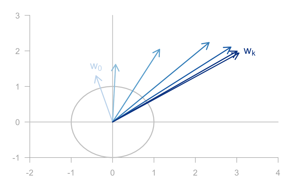
Figure 12.1: Illustration of the sequence of vectors in the Power Method

In practice, we must rescale the obtained vector \(\mathbf{w_k}\) at each step in order to avoid an eventual overflow or underflow. Also, the rescaling will allows us to judge whether the sequence is converging. Assuming a reasonable scaling strategy, the sequence of iterates will usually converge to the dominant eigenvector of \(\mathbf{S}\). In other words, after some iterations, the vector \(\mathbf{w_{k-1}}\) and \(\mathbf{w_k}\) will be very similar, if not identical. The obtained vector is the dominant eigenvector. To get the corresponding eigenvalue we calculate the so-called Rayleigh quotient given by:

\[ \lambda = \frac{\mathbf{w_{k}^{\mathsf{T}} S^\mathsf{T} w_k}}{\| \mathbf{w_k} \|^2} \]

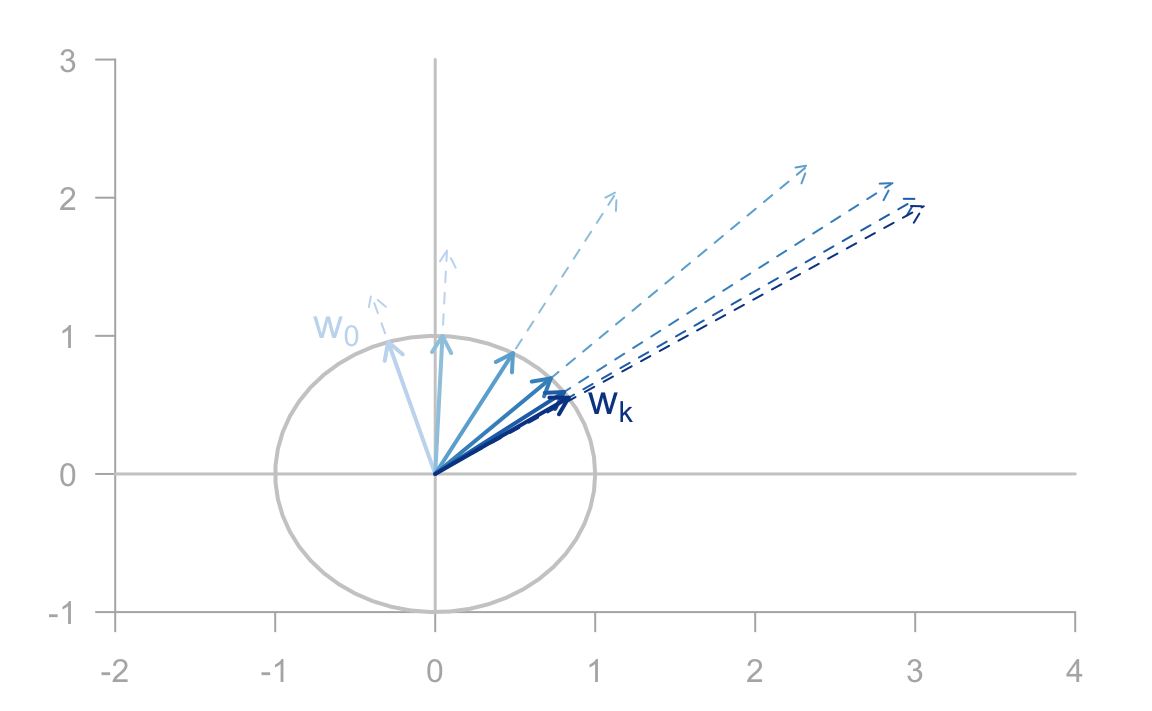
Figure 12.2: Sequence of vectors before and after scaling to unit norm

12.3.1 Power Method Algorithm

There are some conditions for the power method to be succesfully used. One of them is that the matrix must have a dominant eigenvalue. The starting vector \(\mathbf{w_0}\) must be nonzero. Very important, we need to scale each of the vectors \(\mathbf{w_k}\), otherwise the algorithm will “explode”.

The Power Method is of a striking simplicity. The only thing we need, computationally speaking, is the operation of matrix multiplication. Let’s consider a more detailed version of the PM algorithm walking through it step by step:

1. Start with an arbitraty initial vector \(\mathbf{w}\)
2. obtain product \(\mathbf{\tilde{w} = S w}\)
3. normalize \(\mathbf{\tilde{w}}\) \[\mathbf{w} = \frac{\mathbf{\tilde{w}}}{\| \mathbf{\tilde{w}} \|}\]
4. compare \(\mathbf{w}\) with its previous version
5. repeat steps 2 till 4 until convergence

12.3.2 Convergence of the Power Method

To see why and how the power method converges to the dominant eigenvalue, we need an important assumption. Let’s say the matrix \(\mathbf{S}\) has \(p\) eigenvalues \(\lambda_1, \lambda_2, \dots, \lambda_p\), and that they are ordered in decreasing way \(|\lambda_1| > |\lambda_2| \geq \dots \geq |\lambda_p|\). Note that the first eigenvalue is strictly greater than the second one. This is a very important assumption. In the same way, we’ll assume that the matrix \(\mathbf{S}\) has \(p\) linearly independent vectors \(\mathbf{v_1}, \dots, \mathbf{v_p}\) ordered in such a way that \(\mathbf{v_j}\) corresponds to \(\lambda_j\).

The initial vector \(\mathbf{w_0}\) may be expressed as a linear combination of \(\mathbf{v_1}, \dots, \mathbf{v_p}\)

\[ \mathbf{w_0} = a_1 \mathbf{v_1} + \dots + a_p \mathbf{v_p} \] At every step of the iterative process the vector \(\mathbf{w_m}\) is given by:

\[ \mathbf{S}^m = a_1 \lambda_{1}^m \mathbf{v_1} + \dots + a_p \lambda_{p}^m \mathbf{v_p} \]

Since \(\lambda_1\) is the dominant eigenvalue, the component in the direction of \(\mathbf{u_1}\) becomes relatively greater than the other components as \(m\) increases. If we knew \(\lambda_1\) in advance, we could rescale at each step by dividing by it to get:

\[ \left(\frac{1}{\lambda_{1}^m}\right) \mathbf{S}^m = a_1 \mathbf{v_1} + \dots + a_p \left(\frac{\lambda_{p}^m}{\lambda_{1}^m}\right) \mathbf{v_p} \]

which converges to the eigenvector \(a_1 \mathbf{v_1}\), provided that \(a_1\) is nonzero. Of course, in real life this scaling strategy is not possible—we don’t know \(\lambda_1\). Consequenlty, the eigenvector is determined only up to a constant multiple, which is not a concern since the really important thing is the direction not the length of the vector.

The speed of the convergence depends on how bigger \(\lambda_1\) is respect with to \(\lambda_2\), and on the choice of the initial vector \(\mathbf{w_0}\). If \(\lambda_1\) is not much larger than \(\lambda_2\), then the convergence will be slow.

One of the advantages of the power method is that it is a sequential method; this means that we can obtain \(\mathbf{w_1, w_2}\), and so on, so that if we only need the first \(k\) vectors, we can stop the procedure at the desired stage. Once we’ve obtained the first eigenvector \(\mathbf{w_1}\), we can compute the second vector by reducing the matrix \(\mathbf{S}\) by the amount explained by the first principal component. This operation of reduction is called deflation and the residual matrix is obtained as:

\[ \mathbf{E = S - z_{1}^{\mathsf{T}} z_1} \]

where \(\mathbf{z_1} = \mathbf{S v_1}\).

In order to calculate the second eigenvalue and its corresponding eigenvector, we operate on \(\mathbf{E}\) in the same way as the operations on \(\mathbf{S}\) to obtain \(\mathbf{w_2}\).